Public Health Analysis: Using Time to Analyze the Link between Arsenic Exposure and Bladder Cancer

Time plays an important role in many analyses.Let's consider a public health example.Being able to visualize and analyze information over time is critical, especially for diseases such as cancer, which tend to have long latency periods.I am a collaborator on a study underway at the University of Michigan School of Public Health to investigate the relationship between bladder cancer and arsenic exposure.Instead of using a typical GIS, which has no temporal dimension, we use the STIS (Space Time Intelligence System), from TerraSeer.The STIS allows us to not only visualize changing data over time, it also enables temporal analyses through the use of scatterplots and histograms.Below I describe how the STIS is used to assign and visualize an individual's lifetime exposure to arsenic (sometimes termed an "exposure history").

The Study
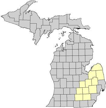
We use information from 220 cases (participants who have been diagnosed with bladder cancer) and 440 controls (those who have not been diagnosed with bladder cancer) from an eleven county region of southeastern Michigan (Figure 1).The controls have been matched to the cases by age (±5 years), race and gender.One goal of the study is to create "exposure histories" for each participant.We want to know how much arsenic (from drinking water) each participant has been exposed to throughout their lives.Thus, we need to know how much water each participant has been drinking, the water source and the concentration of arsenic in that source.There have been no conclusions yet about the correlation between arsenic and bladder cancer.We haven't been able to enroll enough cases yet to draw any firm conclusions.

Figure 1: Study area.The 11 county study area in southeastern Michigan includes (from southwestern corner): Jackson, Washtenaw, Ingham, Livingston, Oakland, Shiawassee, Genesee, Lapeer, Tuscola, Sanilac and Huron.

Participant Data
Each participant answers a written and telephone questionnaire.The written questionnaire asks for each residence lived in for more than a year and the drinking water source at that residence (community supply, private well, bottled water), since each water source has a different arsenic concentration.The telephone questionnaire asks how much water each participant generally drinks each day, and if there were any major changes over the course of their lives (and approximately what year(s) these changes occurred).As an example, Participant A was born in House A in 1950.He lived there for 10 years and drank water from a private well.In 1960 he moved to House B and lived there for 30 years.He drank community water during these years.In 1990 he moved back to his home town and lived once again in House A, but by this time the private well was turned off and the house was on community water.Five years later in 1995 he bought a different house and this is his current address.He is once again on a private well.This participant is currently 55 years old and has had no major changes in his drinking water consumption history.However he did move four times and changed his drinking water source four times.It is these changing spatial and temporal data that STIS can handle.The address information is geocoded using ArcGIS, and a point shapefile is created.The attributes of this point shapefile include:

• ID "" a random ID given to each participant
• start year (mm/dd/yyyy) - the year the participant moved into the residence
• end year (mm/dd/yyyy) - the year the participant moved out of the residence
• water source- the source of the participant's water (private well, bottled"¦).

Figure 2 shows participants at three different time intervals and Movie 1 shows these individuals over an 80 year time period.Notice the gradual change from private wells (in the early years) to community supplies (more recently).Also noticeable is the increase in the number of participants through the years.Using STIS it is easy to see the changes in residences and source of drinking water through the years.

Figure 2: Participants by water source in 1950, 1970, and 2002.Cases are circles and controls are squares.(Click image for larger view.)

Movie 1: [Ed.note: The movies are best viewed in Internet Explorer, using Windows Media Player.] Participants by water source from 1920 to 2002, every two years.Cases are circles and controls are squares.Notice participants moving into and around the study area, as well as their water source changes.

Arsenic Data
As well as geographic location and water source, another important piece of information needed in order to calculate "exposure histories" is the arsenic concentration at past and current residences.At participants' current residences, research staff collected drinking water samples during field visits.The water samples were brought back to the lab and analyzed for arsenic.Every participant was assigned an arsenic concentration for their current residence.In order to assign an arsenic concentration to all the previous addresses however, historical information was collected.Michigan Department of Environmental Quality (MDEQ) maintains a database of arsenic measurements in public well water supplies.

In addition, each public water supply serving a population greater than 1,000 was contacted by telephone to learn their arsenic concentrations. Information was also collected relating to source of supply (ground water wells versus surface water), treatment (carbon filter, reverse osmosis), the geographic extent of the public supply, and how this extent and the characteristics of the source of supply changed through time.

If a change occurred, then the year of the change was noted.For example, the town of Ypsilanti used a ground water well system from 1940-1972.In 1972 it started mixing the ground water from the wells with purchased surface water.Finally it switched entirely to surface water in 1996, and at this time the ground water wells were closed. Therefore, arsenic concentration estimates associated with these modifications in supply also changed accordingly.

Furthermore, a town may experience changes in its geographic boundaries; reflecting population growth.The system will grow as the demand for public water grows.This information becomes part of the public water supply dataset, a polygon layer whose boundaries and values change spatially and temporally.The attributes of this polygon shapefile include:

• Town name "" the name of the public water supplier (generally the town name)
• start year (mm/dd/yyyy) - the year the town started and/or changed its public water supply system
• end year (mm/dd/yyyy) - the year the town ended its change in a particular practice or supply source (i.e.from ground water wells to surface water)
• water source - the source of the public supply water (ground water wells, surface water)
• arsenic concentration estimates "" the estimate from the collected MDEQ and telephone interview (ug/L).

Figure 3 and Movie 2 show the public water supply dataset as its values and boundaries change over time.

Figure 3: Changing mean arsenic values (ug/L) of public water supply systems in the area for 1950, 1970, and 2002.In Genesee County (middle of map) it is clear how the mean arsenic value decreases over the years.(Click image for larger view.)

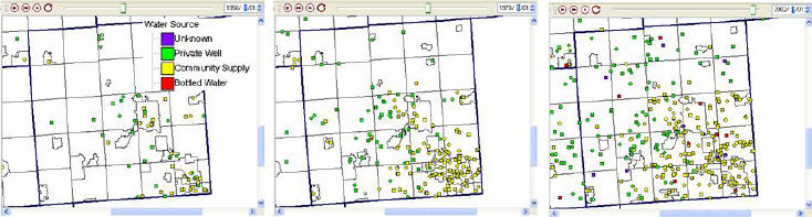
Movie 2: [Ed.note: The movies are best viewed in Internet Explorer, using Windows Media Player.] Public water supply systems in the area from 1920 to 2002, every two years.The upper picture shows the whole study area, the larger screen shows a zoomed in area.Notice the change in the mean arsenic values as well as the public water supply system boundaries change.

Finally, a private well dataset was created using data from an MDEQ database of arsenic measurements from over 8,000 private wells.Unlike the point (residential) dataset and the polygon (public water supply) dataset, this is a raster dataset that does not change over time.

New STIS Data
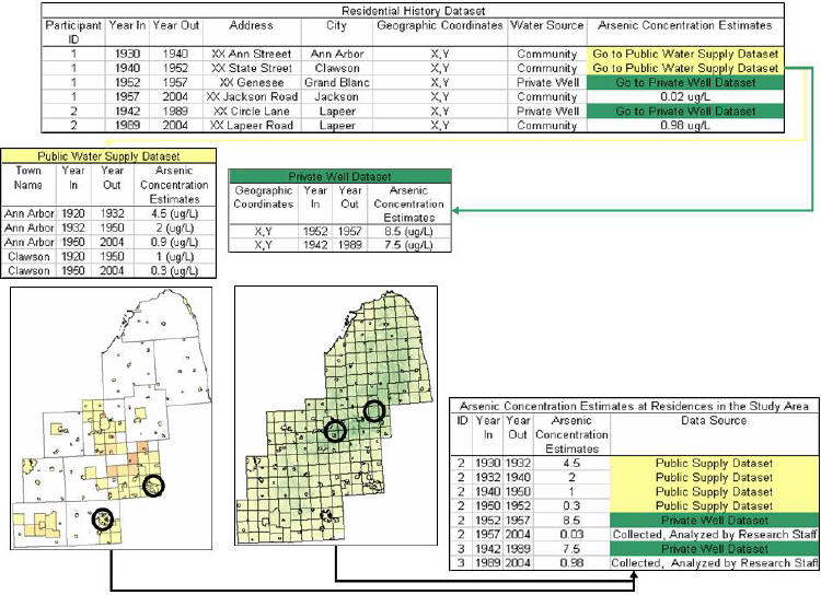
By viewing movie 1 and 2, you can see how the STIS animates spatio-temporal data.But we also used it to handle and create two new datasets "" an arsenic concentration (ug/L) for each participant at every residence and an exposure to arsenic in drinking water throughout a participant's life "" an "exposure history" (ug/day).Recall that we already have an arsenic concentration at current residences.We have values assigned for all current residences and for any time period where a participant drank bottled water.(If a participant ever drank bottled water, the median arsenic concentration in analyzed bottled water samples was used (0.17 ug /L)).We use the two databases (public water supply, and private well raster) to retrieve all other historic arsenic concentrations.The STIS procedure successively loops through each person's residential history, retrieves their water source history and their x,y coordinates, and assigns an arsenic concentration for each space-time interval (Figure 4) using this information.Again, the datasets described above provide the arsenic value for each participant.The STIS is able to determine arsenic concentration estimates based on the changing underlying spatial (x,y of each residence, public water supply polygon boundaries, and raster pixel) and temporal information (year in / year out of each residence and change in public water supply arsenic value).

Figure 4: Flow chart of STIS-based method for assigning arsenic concentrations to past residences and thereby creating a new dataset (arsenic concentration estimates).(Click image for larger view.)

The second dataset created by STIS is the exposure estimate.Again, this value may change many times for each participant depending on whether the arsenic concentration estimates change and/or the drinking water consumption habits change.Movie 3 shows the creation of this dataset.

Movie 3: [Ed.note: The movies are best viewed in Internet Explorer, using Windows Media Player.] Creation of 'exposure histories.' Making sure that an arsenic concentration value is assigned to each participant, a new dataset is created by multiplying the arsenic concentration (including current and past results) by the drinking water value.This information can then be viewed in a table.In STIS, tables can also be animated through the years.Note the change in exposure for the highlighted participants. This change occurs due to a change in source (and therefore arsenic concentration) or a change in drinking water consumption.

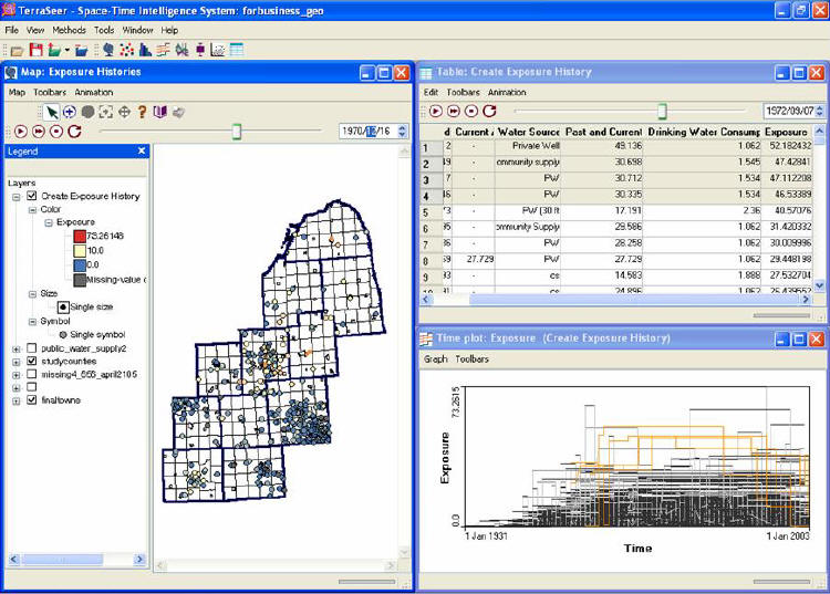
Once these datasets are created, the fun begins.STIS comes packaged with many neat features (Figure 5) as well as a set of spatial statistics.We can now look for clustering of high arsenic values through the whole study area using one of the global clustering statistics or we might be more interested in local clustering of cases in which case we would use the Local Moran.

Figure 5: Linking of maps, graphs and tables in STIS.All participants with an exposure greater than 45 ug/day (in 1970) are selected.By selecting them in the table, they are also highlighted on the map and in the time plot.These participants all live in Genesee or Lapeer County in this time.We can also see a decrease in their exposure in the late 1980's in the time plot of "exposure history." (Click image for larger view.)

Conclusion
The STIS has proven to be a useful tool for this public health project. Although I come from a medical geography background, I can see many exciting applications for STIS in the marketing or business sector.It could be used to:

• Highlight clusters of productive stores over time and estimate new store locations.
• Visualize the boundaries of changing market areas, and inspire new market analysis.
• Analyze socio-demographic characteristics over time for a target spending group, helping a company adjust product placement and target certain stores with certain products in the future.

Ed.Note: BioMedware, the author's employer, is TerraSeer's exclusive research and development partner.

Share