Ed. note: Part one of this article appeared on Aug. 25.
Considerations for Setting Map Road Speeds
Setting the road speeds accurately will really impact the solution. Experience shows that the closer the road speed model is to how drivers actually drive, the better the predictions will be for route arrival times. Enterprise level applications sometimes allow for editing roads to adjust roads speeds on a much more finely tuned basis. Since these businesses cover many states or even the entire United States, they adjust the maps to road conditions locally and sometimes even seasonally.
Remember that travel time includes all windshield time for drivers. Driving, traffic and parking the vehicle all get rolled in to travel time. If drivers spend a lot of time looking for parking, adjusting the road speeds downward may help on the local roads. Traffic, stop signs, traffic lights and any acceleration/deceleration effects hamper achieving the posted speed limit in many cases along local roads and even highways, so setting roads to actual posted limits can make predicted travel times too fast. A general rule of thumb used by some is to set the road speeds at least 10 mph lower than the posted speed for the class of roads. If interstates are posted 55 mph, they may be set to 45 mph. If local roads are posted to 30 mph, set them to 20 mph. This really helps to make calculated arrival times more realistic. In very dense, high traffic areas, setting all surface roads to 10 or 15 mph may work. Several businesses that tried this in New York City were amazed at how the solutions changed and driver satisfaction with routes improved markedly. In rural areas, setting the road speeds closer to the posted limits works very well, especially on interstate, federal and state highways.
Look at Los Angeles as an example. Lots of freeways cross the vast, sprawling metropolis. Unfortunately, those freeways are often clogged with traffic, even on weekends. Many service and delivery companies that work in the city avoid them at all cost. A routing solution should take that fact into account. If an application has hierarchical routing, it probably should be turned off for local routing in general, but certainly it should not be used in an instance like this. Another trick is to reduce the highway road speed settings to match or be even lower than surface roads. Since road speed in a travel time algorithm is treated like resistance in an electrical network or pipe diameter in a flow network, having low speeds on highways increases their"resistance" to being used and will give preference to other roads in the solution. It still allows them to be used in a travel path solution when that is the only option, but it can prevent their general use.
Unfortunately, some very popular forms of map data do not support this level of road speed editing. While customized enterprise solutions often do allow for this sort of editing, many of the out-of-the-box datasets do not allow for this sort of"trickery." The user can still get around some of these data restrictions by resetting the system road speeds and recalculating all or certain routes, while the road speeds are set as needed for the localized conditions. Unless the user is routing for a very large area, problems like those just described may not be an issue.
Many applications now allow the creation and use of barriers in a network solution. Barriers can be placed as points along a road or in polygonal areas of roads that the network will avoid. Closing roads completely can be a problem, so the user has to be careful when using barriers. We will use that same simple city as an example.
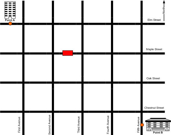
First, let's assume the user adds a barrier to traffic on Maple Street between Second and Third Avenue. Visually, this is what we'd expect:
 |
To get from point A to point B, Maple Street is not available going east to west or west to east between Second and Third Avenue. The routing solution will avoid this block by going around the barrier, but it can still reach pretty much any place on Maple Street.
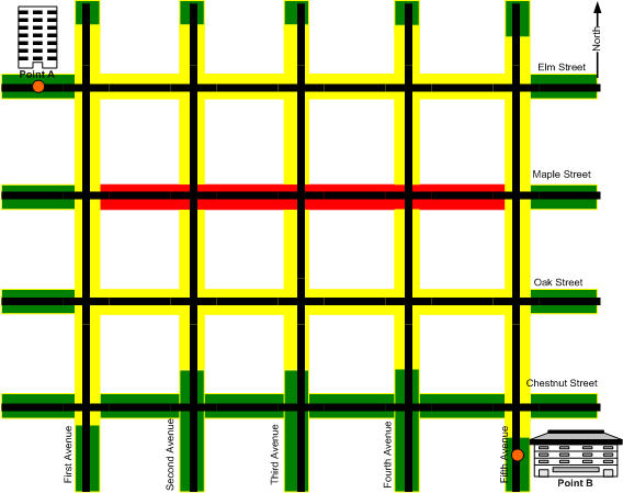
If we place a barrier along a length of Maple Street, no part of Maple Street along the barrier can be visited. This may be realistic when roads are closed and cannot be traversed, but routing solutions are too smart. They will take this barrier literally and not route to any stops inside the barrier.
 |
No addresses that geocode in any of the ranges along the red barrier can be visited by the routing solution. While that may realistically show what is happening along the street, the driver would, in most cases, park down the block or around the corner to visit a stop inside that barrier. Using barriers that close more than a point in a network can cause problems if you have stops that must be visited within the barrier. Some applications will leave the stops unrouted because they cannot be reached (and some older ones may even time out processing in an infinite loop trying to visit an unreachable point!). Most routing systems cannot even route those manually because they can't calculate a travel time to the point. The order can be placed on a route but it will not sequence or recalculate an ETA with a stop in a barrier. Anytime there are incongruities in the road network where stops cannot be reached, problems may occur. If barriers are used, point barriers tend to be the safest approach.
There is another alternative to barriers that some businesses use successfully in their routing applications. Instead of precluding traffic on a set of roads, set the roads at a very, very low road speed. If the system allows setting individual road speeds, the user can select an area of road and set it to, perhaps, 5 mph. That way the system will preferentially route drivers around the lower speed roads. This can be useful for festivals, parades and other events that impact areas of a city or town. In our simple example, assume there is a festival for a few days along and near Maple Street for a few blocks. The user may want to allow services, deliveries or pickups in that area but may generally want drivers to avoid that area. The user can select Maple and the two parallel roads to the north and south for a few blocks to denote the festival area and set the road speed to 5 mph. If the system tries to route from point A to point B, you can be pretty certain that it will recommend a right off Elm Street and driving down First Avenue to the south and then east on Chestnut Street to Fifth Avenue, because their assigned speeds are higher than the area of the festival.
 |
The type of vehicle may also force different road speed settings. A small van usually has no problem traveling as fast as a car. A 55-foot trailer being towed by a rig may not proceed as quickly as a car or van. Road speeds and vehicle types are another consideration.
Weather and seasons present another set of map considerations. Maps for mountainous territory should probably have lower road speed settings in winter than in summer. Rainy seasons require drivers to proceed more slowly. The effects of large storms may last for days and modifying road speeds might be critical for both business and municipal routing applications.
All of this editing mentioned above is just an attempt to emulate real road and traffic conditions. There are several services available that often partner with map vendors or are available on their own that can provide traffic data. Traffic data come in several varieties. Real-time traffic data take inputs from metropolitan and large suburban areas where traffic information is available and feed these into the traffic providers' database. From there they can be delivered, accessed or streamed to the users' environment. Historical traffic is also available. Lastly, predicted traffic is the newest form of data available to users.
Live Traffic Inputs to the Map
Using live traffic can be very beneficial and very tricky at the same time. The problem becomes, what are you going to do with the information once you have it? A driver who knows where the traffic is can adjust his driving to try to avoid traffic problems. That can be a very good thing and that information is easily delivered to vehicles via cellular technology. Trying to use that information in an application is a more difficult undertaking. Extending or contracting an existing route is fairly simple; take the current traffic condition, apply a road speed to that and recalculate the existing route's arrival time at each stop. Few applications do that, but it is technically feasible and can be done rather simply if the road speed database is modifiable or if the system can use an alternate input for road speeds.
Extending the use of live traffic into a routing solution now introduces a new level of complexity. Certainly the route can be rerun with the dynamically new road speeds, but are the users and drivers willing to have new routes based on these dynamic road speeds? Probably not. If road speeds vary from an initial prediction, the recommended assignment of stops will change from vehicle to vehicle and that is usually not acceptable to most businesses or municipalities. It may be useful for new work assignments, but existing work assignments need to stay on the vehicles to which they are currently assigned.
 |
Historical and Predictive Traffic Inputs to the Map
Historical traffic can introduce a beautiful concept - time of day corrections to road speeds. This sounds like a great innovation, particularly in creating routes. In one respect, it is. In another respect, it can be a nightmare. Let's look at the benefit first.
Providing a good average road speed for a network is a great feature of historical traffic data. Getting the best overall data into the map data to be utilized in a routing application is of great utility. Trying to model the routes as the driver navigates from stop to stop over the course of a day is a good thing.
On the other hand, time-of-day road speeds become cumbersome and really hinder the calculation of routes. Most applications assign work through a matrix of stops and their interrelationships. That matrix now has to include all the possible time-of-day effects for travel time, so the matrix explodes into a very large and unmanageable entity, impossible to calculate in a reasonable amount of time. It can be managed by using average road speeds to calculate the matrix, and then extending and contracting existing routes based on time-of-day effects on road speed, but few systems, if any, currently can do that.
Lastly, predictive road speeds based on current traffic are available. Those take the dynamic traffic as it is now and use some sort of fairing calculations to get the dynamic conditions back to historical. Problems with that are included in both of the prior option discussions.
Predicted Versus Reality: Summing it All Up
The user has to remember in all this that the routing system is giving him an estimate of what the route may look like. Realistically, once the first vehicle leaves for the day, what that vehicle is actually doing will never perfectly match the predicted route. Estimating travel time is part science and part art. Who knows how many red lights an actual driver will hit as he travels between stops? On average, drivers will hit around half of them. A very few will hit none or all of them. Most will hit a few. Some will take the average time between stops here and there, but most will not, exactly.
Additionally, the systems that route also take into account a given stop duration. That, too, is an average. A stop estimated to take 10 minutes can vary based on how far the customer is from the parking location, both horizontally and vertically in multi-story buildings; how long it takes the customer to answer the door; how long it takes to really do the work at the stop; how long it takes to do any additional paperwork/customer charges at the stop, and then return to the vehicle. A 10-minute scheduled stop may only last a minute for a not-at-home customer or hours for a customer with unexpected issues.
Creating routes and vehicle arrival times has a lot of artistic guesswork associated with it. The amount of maintenance required for maps is based on how critical it is for a user to try to model all or some of them, realizing that they are inherently inaccurate once reality sets it. The best you can usually hope for is to take an average, conservative approach to road speed and time duration estimates and use them as a predictor. As customers gain experience using their routing applications, tweaks and changes and improvements can be made, but you always have to consider what is gained for the costs incurred in trying to do more.
As we have shown, the map plays a large role in how the routing solution will look to the user and driver between stops. The path the system takes should mimic how drivers are actually expected to drive, especially if the system provides them driving directions. While maintaining a map is not as simple a problem as you might have thought, it is not"rocket science." With a little common sense, the map and its underlying road network can be maintained to give users the result they need to run their business or operation.