Convolution: Part 3 of 3

(Part Three of a Three part series - ed.)

5. Putting it all together

The FFT algorithm itself is pretty simple (the core routine in Numerical Recipes requires less than a page of Fortran) and is a part of many software packages and code libraries. (Intel offers a numerical analysis library including several kinds of FFTs for free.) Unfortunately, FFT is not a part of Spatial Analyst. Usually it is found only in image analysis packages.

The Spatial Analyst developers have been far-sighted in providing an object library for incorporating other programs into Spatial Analyst itself. (This is the “gridIO” library referred to earlier.) I used it to build the FFT right into Spatial Analyst. Doing this was an adventure in its own right, but one more suited for discussion in a mixed-language or numerical programming course. (I used a high-performance Fortran compiler for the dirty work.) At the end, though, I had a new Spatial Analyst request that performs Algorithm 2. You provide it two grid data sets (input and kernel) and it creates the convolution as a new grid data set, suitable for immediate display and post-analysis in ArcView.

Using this new capability, Hoogerwerf performed the convolution operation on his 550 MHz machine in 22 seconds. Eight of these seconds are for reading the input grid and writing out the result. (The actual grid is 1,920 rows of 1,680 cells each, requiring 1920 * 1680 * 4 = 12.3 MB, because each cell needs four bytes.) The other 14 of these seconds do the computation in double precision, assuring high accuracy. In short, the computation time is comparable to the time needed simply to copy the input grid to an output data set. It’s hard to do much better than that.

Or is it? Earlier I rejected one of the design choices—the so-called direct method—because its execution time in Spatial Analyst was three hours or more. Having learned in the meantime how to interface high-performance code with Spatial Analyst, it seemed worth a few minutes to consider what the direct method might do. To my surprise, the calculations suggested it would run even faster than the FFT.

As I have implemented it, the direct method uses the same input as the FFT. You convert the farm emissions data into a grid (that’s a one-step operation) and you construct a kernel grid to describe the deposition behavior (that’s much trickier and involves some techniques worthy of their own discussion at a later time. But it only has to be done once!). The calculation is by brute force: each input cell gets spread according to the kernel into the output cells and accumulated there. But this time, expecting only a tiny fraction of the input cells to have any data (the others are just space between farms), we first test that the input cell has a nonzero value. If it does not, we just move on to the next cell.

Ordinarily, this approach does not save any appreciable time. A general-purpose convolution function has to be able to process input grids that have data everywhere. (I will give you some examples shortly.) In this case, though, we already have a general-purpose function in the form of the FFT. We can afford first to inspect every cell in the grid. If enough of them are zero, we apply the direct method. Otherwise, we fall back on the FFT. As a result, Hoogerwerf’s calculation can be done not in 14 seconds (plus grid I/O), but actually in 8 seconds. That’s good enough for me, and he seems pretty happy with it too.

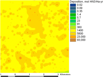
A small portion of the model output. It corresponds to the input shown previously. Note the logarithmic scale.

6. Where do we go from here?

It is satisfying to reduce a computation from a matter of hours to a matter of seconds—it’s a little like flying a turtle at supersonic speeds. But if this approach worked only for the problem at hand, it would not be very interesting. What make it valuable are all the other possible applications.

Here are some examples of what a fast convolution procedure can do.

Image analysis. Most image analysis functions involve small kernels ranging from 2 x 2 to 5 x 5. But some do not. The “Gaussian blur,” for example, can require arbitrarily large kernels. We can now do these in seconds in Spatial Analyst.
Data smoothing. Grids of data often require smoothing to make spatial patterns more evident, to reduce artifact-producing noise, and as a preliminary to calculations of slope, gradient, aspect, curvature, and more. Many sophisticated smooths are convolutions using extended kernels.
Density calculations. Spatial Analyst offers a density estimator with two kernels—a constant kernel and a quartic approximation to a Gaussian kernel, but it works only with point data sets. With a full-fledged convolution function you can choose any density kernel you like and rapidly perform the computation on any grid, including those derived from linear and polygonal features.
Surface analysis. Computations of derivatives (slopes) are convolutions. Using appropriate kernels you can simultaneously smooth a surface and derive these surface functions.
Solution of dispersion models. Models of air emissions and of many other advective and diffusive phenomena have solutions expressible as convolutions. Usually the kernels are quite large.
Signal processing and digital filtering. These are sophisticated forms of smoothing that frequently use large kernels.
Assessment of spatial correlation. Most traditional statistical methods do not give appropriate answers when applied directly to gridded data. One problem is that data tend to be strongly correlated from cell to cell. To compensate for this, many correlation coefficients must be computed—one for each possible displacement of a cell relative to its neighbors. This produces a grid of correlation coefficients. It can be efficiently computed by convolving the original grid with a version of itself (produced simply by rotating it 180 degrees).
Assessment and representation of uncertainty. By converting spatial features, whether polygonal, linear, or point-like, and convolving with a probability kernel, you can visually indicate locational uncertainty. High uncertainty requires a large kernel.

7. Principles

Understanding how your software works can provide crucial information for the design of a solution. We would have been stuck at the very beginning without having a good appreciation for the alternative ways of expressing convolutions. Our calculations of processing time, which helped suggest other solutions, would have been difficult or impossible.

Choices of data structure and algorithm usually are much more important to the performance of a solution than choice of hardware or software platform. You can buy a supercomputer with 1,000 processors and achieve a speed up of less than 1,000. Choosing the right algorithm and a good data structure (the grids, in this case) gave us a solution more than 1,000 times faster.

Undertaking a careful analysis of computing requirements early in the design process often pays off. It became clear early on that time was the constraint. RAM can become a constraint for the FFT, but the direct method can be implemented using remarkably little RAM. You could cover all Europe with a 25-meter grid (it would have 100,000 or so rows and columns) and still run the direct algorithm comfortably in 128 MB.

Selection of a solution method depends on the user’s requirements. It is usually pointless to speed up something that is fast enough or to reduce memory requirements when RAM is cheap. It was helpful to understand that the intended use of the computation was for repeated interactive analysis. In other situations we would have arrived at a completely different solution.

One mark of a robust and powerful software platform is its extensibility. I am comfortable committing projects to an ArcView + Spatial Analyst platform because if I run into some unusual need I know it can be accommodated and that there will likely be many solution options available.

It is not enough just to be clever; far better is it to build on what other people have already discovered. The GIS is a powerful tool, but it truly comes into its own when used by an analyst who has a strong theoretical background and the ability to learn from the literature.

____________________

Addendum

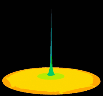
The deposition kernel in spatial perspective. Reproduced courtesy Marc Hoogerwerf.

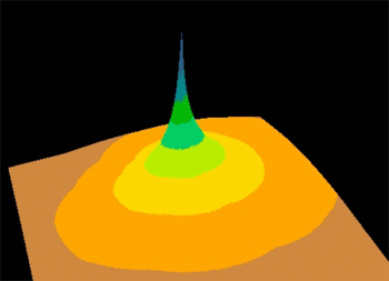
Spatial perspective of another deposition kernel. The model described in the article is merely the simplest in a hierarchy of possible models. The more complex ones use kernels that vary from point to point depending on local meteorological data. Reproduced courtesy Marc Hoogerwerf.