Cowpacity: A Grazing Carrying Capacity GIS Model

Background

In the GIS world of environmental consulting it is not often that an opportunity to build a complex model that is both challenging and exciting to develop comes along; the Cowpacity GIS model offered that opportunity. Currently WRA Inc. has run the model on six different properties in the Bay Area. We hope that outreach efforts to open space preserve and other rangeland area managers will result in additional opportunities to deploy the model. Given the automated nature of the modelbuilder environment (only the gathering of input GIS layers are required to run the model), the Cowpacity GIS model provides WRA Inc.’s clients with a scientifically-based product that is also very economical.

Many preserved lands require prescribed livestock grazing as a management tool to promote healthy habitats for protected species, control invasive weeds, and/or reduce fire hazards. WRA Inc. has prescribed and facilitated grazing on numerous sites throughout California, conducted infrastructure design, Residual Dry Matter (RDM) monitoring, and rotation planning for the purpose of improving specific special-status wildlife or plant species habitat. In order to provide accurate calculations as a basis for making prescribed grazing recommendations WRA Inc. created Cowpacity, a carrying capacity GIS model to help quantify optimal grazing regimes. The area of interest in this article is a conservation bank located in Santa Clara County that is home to several rare species which depend on sound grazing practices.

Carrying Capacity Calculation and Terminology

The equation for carrying capacity is: Production - Target RDM / 900 = Animal Unit Months (AUM). Production is the annual estimated production of range forage (Lbs/acre) for favorable (high rainfall) and unfavorable (low rainfall) years. Target RDM is the recommended amount of above ground plant material (Lbs/acre) at the beginning of a new growing season which protects against erosion and loss of soil nutrients. Targets are based on recommendations published by the University of California (Bartolome, et al 2002) (Table 1). The divisor 900 is the estimated amount of dry forage (Lbs) consumed per animal unit in a month. AUM is the number of animal units that could be supported by the estimated available dry forage for one month (e.g. 10 AUM = 10 cows in a grazing unit for 1 month or 1 cow for 10 months). An Animal Unit is a standard measurement that is based on a single 1,000 pound cow; however different animal unit equivalents can also be used for different types of animals (Table 2).

GIS Data Inputs

Grazing Units: delineated from surveyed pasture fence lines.
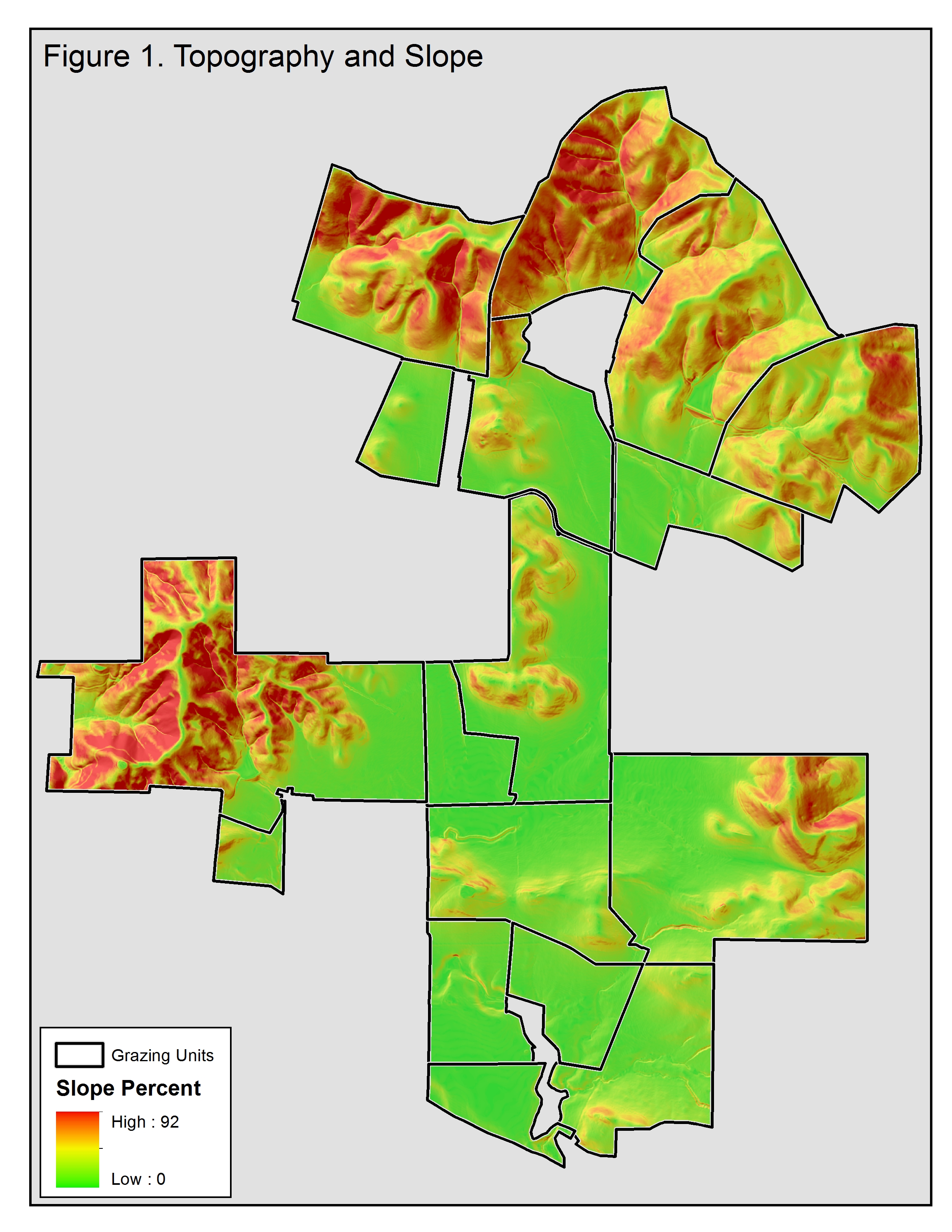
Digital Elevation Model (DEM): interpolated from 1' LiDAR contours downloaded from the Santa Clara Valley Water District. Slope (Figure 1), slope restrictions (Table 3), and other surface calculations are derived from the DEM.
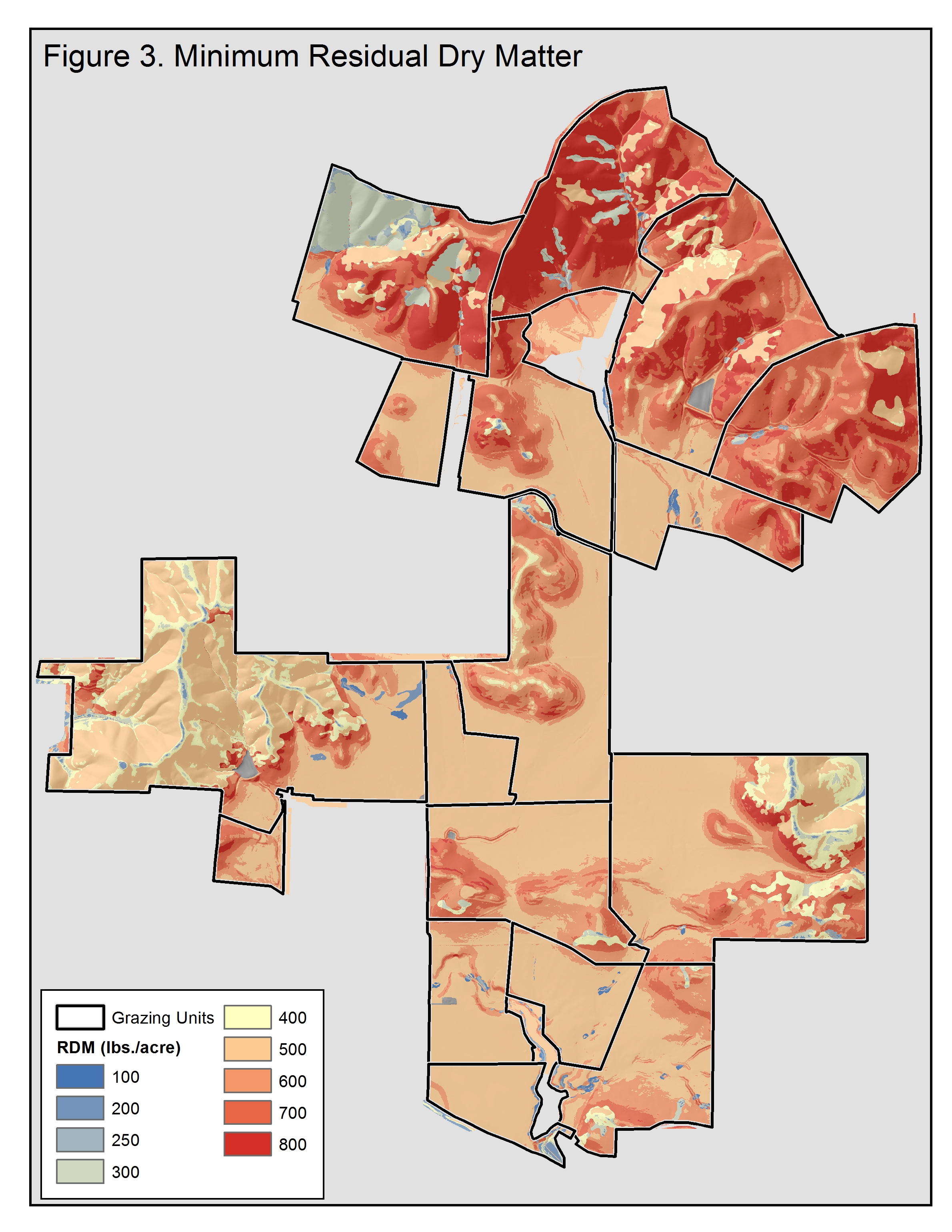
Woody Cover: derived from site specific vegetation map surveyed by WRA Inc. (Figure 2). RDM is calculated from a combination of slope and percent woody cover (Table 1 and Figure 3).
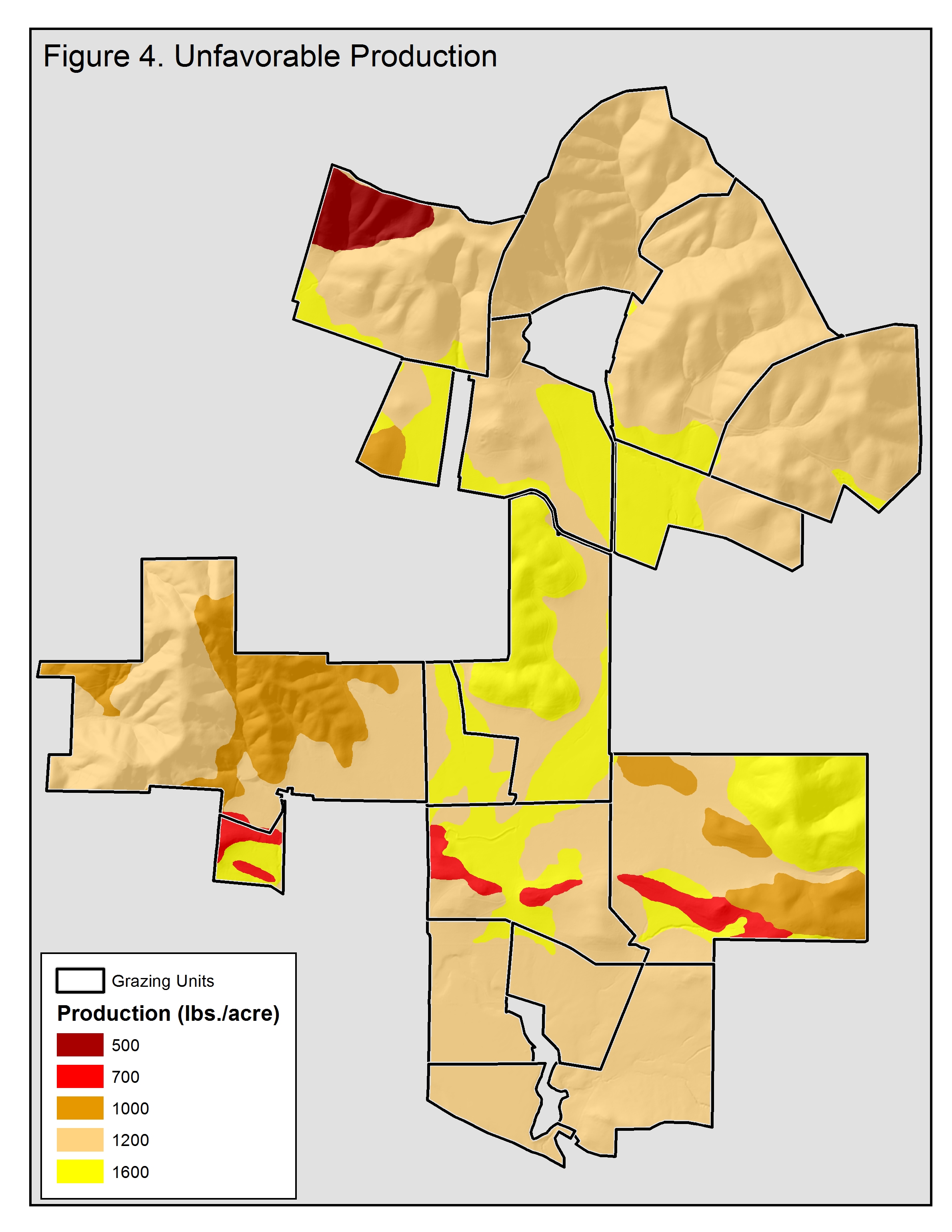
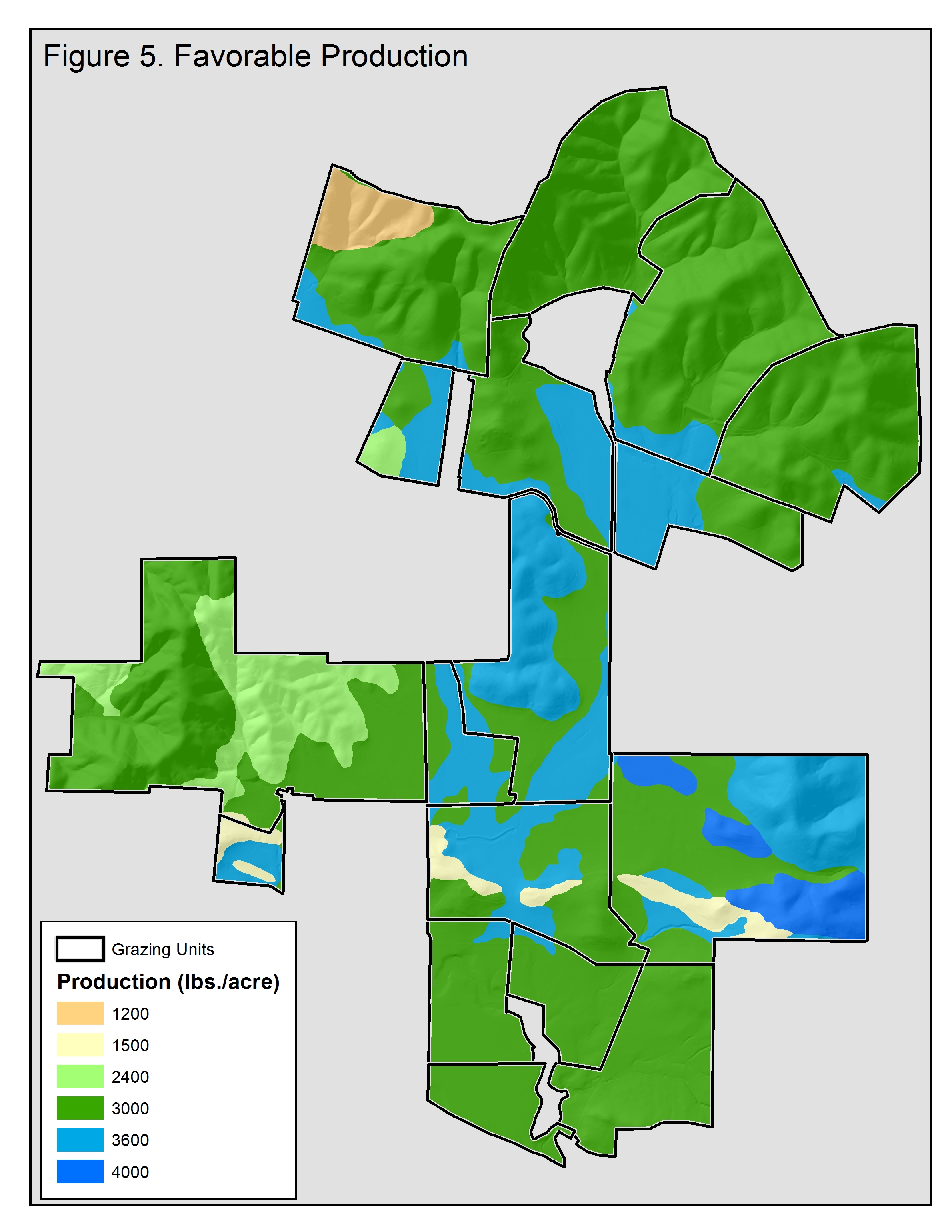
Production: NRCS SSURGO soils database which includes both favorable and unfavorable production values within its attributes (Figure 4 and Figure 5).
Available Water: surveyed locations of troughs, stockponds, or natural springs that livestock use for water sources. The values from Table 4 will be applied as restrictions to AUM values (Figure 6).

The Model Approach

ESRI Modelbuilder is used to calculate AUM for the entire project site using primarily raster-based analysis; Zonal Statistics summarizes AUM calculations per grazing unit. The model also accounts for actual surface area (versus pure planimetric x, y geometry) for AUM calculations in order to be topographically correct and increase accuracy.

Cowpacity Model Order of Operations

Slope Percent is calculated from Elevation, and then reclassified to values in Table 1.
Woody Cover is rasterized using values in Table 1 then added with Slope Reclass to create an index that can be reclassified to RDM values.
Soils data is rasterized to Production values then subtracted by RDM to get Total Production.
Two restriction values are applied to reduce Total Production:
- A second Slope reclassification according to restrictions in Table 3.
- Path Distance tool from Available Water is applied using values in Table 4. Path Distance also uses Elevation to derive actual surface distance. In order to contain the Distance From Water raster within each grazing unit, a Cost raster is used within the tool to make fence lines too costly to pass through.
A conditional statement is used to turn negative values to '0' (these are areas that either have unsuitable vegetation for grazing or exceed thresholds in Table 3 and Table 4).
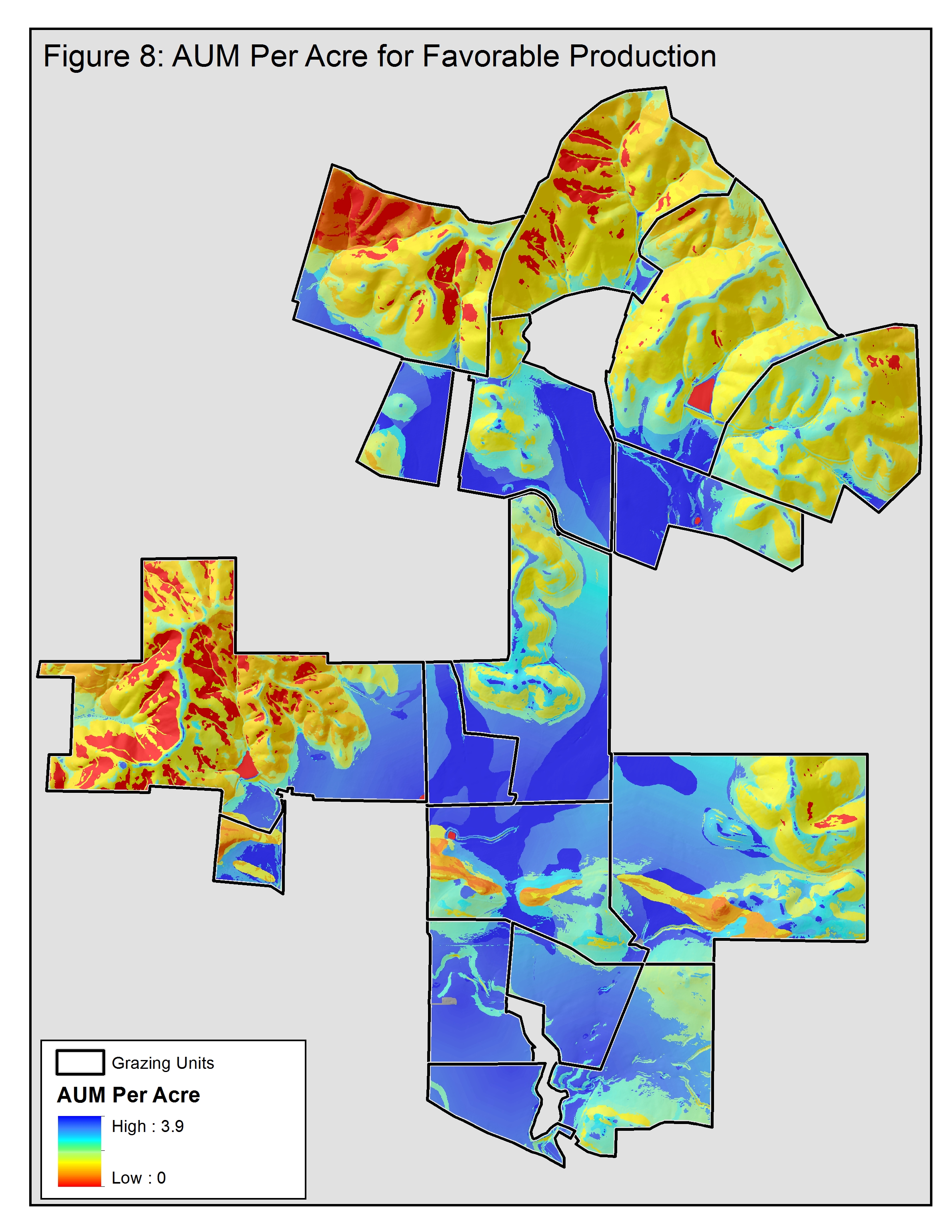
The divisor 900 is applied resulting in AUM Per Acre (Figure 7 and Figure 8).
Calculate percent acre per pixel resolution resulting in AUM Per Cell.
Apply geometric equations (using Slope Degree and cosine functions) to arrive at the actual surface area per cell versus a strictly planimetric area.
Use Zonal Statistics to summarize AUM per grazing unit, and then calculate those values into the grazing unit table (Table 5).
The model is run for both favorable and unfavorable production years.

Model Diagram for Favorable Year (click for larger image)

Conclusion

WRA, Inc. hopes to streamline the process by identifying production and RDM values at the county level, however, fence lines and water sources for livestock will always need to be based on site-specific mapping. Since its inception we have continually made improvements and as such we perceive the model to be adaptive and flexible. The earliest version only did the basic AUM calculations, but over the last few years we added the additional slope and distance from water source restrictions in order to factor in livestock behavior. Additional factors that could be added to account for cattle behavior are shade sources and prevailing winds, to name a few. Additionally, comparison of model output to actual stocking rates, site productivity, and RDM will be used to further calibrate the model and allow replacement of SSURGO soils database with more accurate regional or site specific estimates of production values.

References

Table 1 - Bartolome J.W., W.E. Frost, N.K. McDougald and J.M. Connor 2002. California Guidelines for Residual Dry Matter (RDM) Management on Coastal Land Foothill Annual Rangelands. Rangeland Monitoring Series, University of California Ag and Nat Res Pub 8092. Oakland, CA. 8 p.

Table 2 - George, Melvin R. 1987. Animal Units, Planning Guide No. 4, Rangeland Watershed Program. U.C. Cooperative Extension and USDA Natural Resource Conservation Service.

Table 3 & 4 - Holecheck, J.L. 1988. An Approach for Setting the Stocking Rate. Rangelands 10:10-14.

Reprinted with permission, The Bay Area Automated Mapping Association (BAAMA) Journal and courtesty of WRA Associates.