The analysis of markets leading to the
decision of choosing the right location for a retail or service
facility has never been an easy task for business decision makers.With
GIS technology, it is much easier and faster to analyze large volumes
of consumer demographic and socioeconomic data and integrate them with
business characteristics, such as sales, location of customers and
competitors.The purpose of using GIS is to produce useful information
from the input data to support the decision making process.Many firms,
and especially retail, have benefited from using GIS technology, while
many others still have to discover its usefulness for their business.
The analysis of markets can be performed at three spatial levels (Ghosh, McLafferty, 1987).They vary from the regional scale (metropolitan areas, cities, towns, etc.), where areas with the greatest market potential are found, to the local scale in which specific sites for locating new stores are evaluated.
The first level involves the examination of such factors as population size, population projections, demographic and socioeconomic characteristics of the population, income and existing competition. Based on these factors, conclusions can be drawn regarding the market size, structure and saturation.
The second level of market analysis determines the spatial differentiation of market potential within a selected city or metropolitan area.The extent to which demographic and socioeconomic characteristics of the population match the profile of firm's target market is studied at this level, along with such factors as land use/zoning, housing patterns, travel and shopping patterns, transportation networks, etc.The analysis of the competition must also be included at this level, resulting in the list of sub-areas ranked from the point of view of the suitability for a business expansion.
The third level of market analysis is site evaluation.Its objective is to prepare a list of potential sites from which the best site can be chosen.There are various approaches to retail site evaluation, ranging from simple ones such as ranking, to complex ones such as the location-allocation modeling.Each of these approaches involves the idea of key factors - variables essential to a firm's success.GIS can be used at all levels of spatial analysis of markets.
The site evaluation process for the chain, or network of stores or service facilities is much more complex than for an independent facility.This is because the addition of a new store affects the entire network of stores.The evaluation of these impacts requires testing multiple scenarios using such techniques as, for example, location-allocation modeling integrated with GIS.
Another challenge for analyzing a network is to answer the question whether or not to enter a new market or expand in an existing one.Many economic reasons (minimizing per-unit marketing, distribution and management costs, gaining strong market presence) indicate that re-evaluating existing markets is more important than identifying the new ones (Munroe, Nurani, 1999).
This article illustrates how GIS technology, combined with some statistical analysis, can be used for identifying potential markets for the hypothetical business - a live music bar.Two approaches are applied: multiple linear regression and suitability modeling.The target variable that is modeled using the regression is the Expenditure on live staged performances as percentage of spending on spectator entertainment performances.In suitability modeling the target variable becomes one of the most important criteria for the analysis.The analyses presented in this article correspond to the second level of market analysis that includes the study of spatial differentiation of market potential within selected metropolitan area, in this case study, Halifax-Dartmouth, Nova Scotia.
Selecting variables for analysis
In the process of finding potential markets, there is usually an abundance of available data.Potential input variables should be extracted from such data sets as Census, consumer spending categories, and point data sets representing location of competitors or location of other important facilities.Selecting the most suitable and relevant variables for further analysis is time consuming but critical.After preparing a long list of potential variables, some criteria should be applied to shorten the list of candidates for variables that will be used as predictors.
The first criterion is to choose variables that are spatially differentiated.The coefficient of variation, which is the ratio between the standard deviation and arithmetic mean, can be used for this purpose.However, all variables (the initial list included sixteen of them) selected for this case study showed similar level of spatial variation and this criterion alone did not help in eliminating some of them.
The second criterion is to analyze how significant is the correlation between a potential predictor and all target variables.Based on this criterion, two potential predictors were eliminated: the density of population and the sum of distances to universities.All other variables revealed a very significant correlation (at the significance level 0.01) with the target variable.
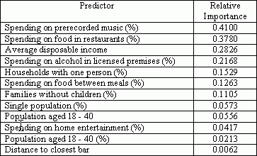
The next approach was to use a neural network algorithm for showing the relative importance of predictors.Table 1 presents the order of predictors according to their importance determined by the neural network algorithm.The most important predictor is the spending on prerecorded music (%); the least important is the distance to closest bar (competitor).
Predicting spending on live staged performances using a regression model
The most common approach to predicting the target variable (Spending on live staged performances) is to apply a multiple linear regression model.The stepwise method was used for entering and removing independent variables from the regression model.This method revealed that the following variables entered the model in the following order:
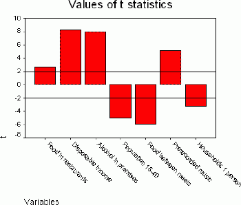
Figure 1.Strength of predictors. Click image for larger view.
It is expected that all independent variables from the regression model are significantly correlated with the target variable.However, collinearity occurs if these variables are inter-correlated among themselves.The tolerance coefficient can be calculated for each variable and used for measuring the collinearity.This coefficient is calculated as the difference 1- R2, where R is the multiple correlation of a given variable with all other independent variables.If this coefficient is close to zero, a problem with collinearity exists.As demonstrated in Figure 2, the tolerance coefficient differs from zero for all the variables, therefore all of them can be used for determining the market potential.However, spending on food in restaurants and spending on prerecorded music has the strongest correlation with other variables, whereas the percent of population aged 18 - 40 has the weakest correlation.
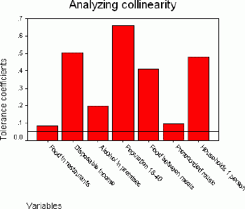
Figure 2.Coefficients of tolerance.Click image for larger view.
The regression model used for predicting the target variable has the form of the following linear equation:
Predicted target variable (Spending on live staged performances %) = -1.735 +
+ 0.155(Spending on food in restaurants %) + 0.00014(Average disposable income) +
+ 0.228(Spending on alcohol in licensed premises %) +
+0.0546(Population aged 18-40 %) - 0.485(Spending on food between meals %) +
+ 0.293(Spending on prerecorded music %) - 0.0467(Households with one person %)
This model is very efficient for prediction, since the correlation between the actual and predicted values is very significant (R = 0.916).Even if actual values are close to predicted, in some areas these residuals (differences) can be significant.If actual values are higher than predicted ones, the market is over-performing and there are some factors that should be found for explaining this phenomenon.If predicted values are higher than actual ones, the market is under-performing and such areas can be considered as untapped market potential.Because residuals are unique for each spatial unit (polygon), they were first standardized and then reclassified into four categories (Table 2).High negative residuals represent untapped market potential good for business.Low negative residuals correspond to moderately good areas for the business expansion.The positive and high positive residuals represent over-performing markets and indicate, respectively, medium low and low market potential (Figure 3).
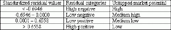
Table 2.Correspondence between residuals and market potential categories. Click image for larger view.
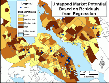
Figure 3.Untapped market potential based on residuals from regression. Click image for larger view.
Analyzing areas with high untapped market potential
In order to perform further analyses, the variables (predictors) were also classified into four categories (low, medium low, medium high and high).Earlier analysis revealed that there is a very significant correlation between each predictor and the target variable.At this point, the question arises: is there a significant association among these variables after they were recoded into four categories? A cross-tabulation was performed for analyzing the association among every predictor and a target variable, each having four categories.The chi-square statistic was used for testing the significance of the association.All associations are significant.Each cross-tabulation resulted in a 4x4 table.The most interesting cell in each 4x4 table is one corresponding to 'high' untapped market potential and category 'high' for each predictor.Table 3 presents the percent of occurrences for each predictor for 'high' / 'high' categories.For example, within the areas representing the high untapped market potential, there are 52.9% occurrences of areas representing high spending on food in restaurants, but only 10.3% of areas with high average disposable income.If the distribution is uniform, the expected value would be 25% (100% spread evenly over four categories).High values for all predictors, except for the disposable income, show higher concentration in areas with high untapped market potential.

Table 3.Comparison of category 'high' of untapped market potential with category 'high' for all predictors. Click image for larger view.
Untapped market potential vs.geodemographic segments
Identification of geodemographic segments that exist in areas with high untapped market potential can help make business decisions by focusing on such segments.On the other hand, if a given geodemographic segment corresponds mainly to areas with low untapped market potential (high positive residuals), that segment should be avoided when considering a location of a given business.Canadian PSYTE clusters were cross-tabulated with four categories of untapped market potential.In areas with high untapped market potential there are 12 different PSYTE clusters, and six of them can be found only in this category.In areas with a low untapped market potential there are eight PSYTE segments and one of them can be found exclusively in this category.These segments should be avoided.More comments on the relationship between clusters and results of modeling can be found in the section titled "Weighted suitability categories vs.geodemographic segments."
Suitability modeling
Suitability analysis represents one of the most common GIS modeling techniques.Some of the factors that make it so attractive include:
The main components of the modeling methodology for determining suitability include the following steps, which will be further discussed below.
1.Define the model
3.Run the model: combine suitability ranks with suitability weights to calculate the final score
4.Analyze the results and present them to the decision makers
The problems for which models are developed can be of various complexities.A team discusses all of the issues associated with the problem being modeled.The complex problem has to be often broken down into smaller problems.Therefore there is usually one general goal and many sub-goals in the model.
In this article, the task is relatively easy to model.The goal is to find the most suitable areas for locating a live music bar.In order to achieve this goal, potential markets will be evaluated using relative suitability scores.Every area included in the analysis will get a suitability score assigned and areas with highest scores will be considered the best ones.
Select variables for analysis and get the data
The selection of criteria for analysis and corresponding data is an integral part of model definition.For this case study, a range of variables describing demographic, socio-economic and lifestyle characteristics of the consumers was selected.Let us assume that a team of experts selected the following variables.
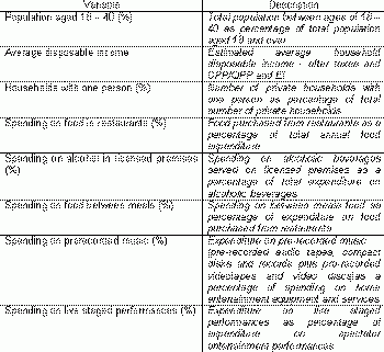
Table 4.Variables for suitability analysis.Click image for larger view.
An ideal customer of the live music bar would then be 18 to 40 years old, a single, with a pretty good income that would allow for certain spending habits listed in Table 4.
Reclassify data into suitability ranks and develop weights
This is the hardest and most subjective part of the modeling methodology.Because the data for the analysis is usually on different measurement scales (nominal, ordinal, interval, ratio), it is impossible to combine data mathematically without placing it on a common scale.Assigning ranks to original data values is a typical solution for bringing data to a 'common denominator.' The original data is converted (reclassified) into new values - suitability ranks -- using experts' judgments.Also weights must be developed to indicate the relative importance of different criteria.Is the age of consumers more important than an average income in the case of locating a live music bar? Assigning ranks and weights is based on preferences. Therefore this step should be completed by a group of experts rather than by a single expert.
One of the group preference assessment techniques is the Delphi method. There is a long tradition in combining the Delphi method with GIS.The purpose of applying this method is to find a group's average preference for assigning ranks and weights.Three characteristics of the Delphi method distinguish it from other preference assessment techniques (Dickey, 1978).
The assessment of relative importance of different criteria is even more critical than the assignment of ranks.The development of weights should always be a team effort.The weights can be changed to increase or decrease the importance of various suitability criteria.The model can then be re-run to produce alternative results.Weights must add up to 1.For this case study, the following weights were chosen.
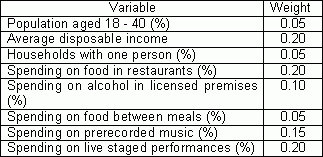
Table 5.Weights for suitability criteria.
It was felt that income, spending on food consumed in restaurants, spending on live staged performances and prerecorded music were more important than the other four variables.
Run the model: combine suitability ranks with suitability weights to calculate the final score
The suitability model was run twice: without weights and with weights. In the first case, variables reclassified into five categories were added together to get a cumulative suitability index.This cumulative suitability index was further reclassified into four categories: high, medium high, medium low and low.Figure 4 illustrates spatial differentiation of suitability categories.The map also displays locations of existing bars in the study area.
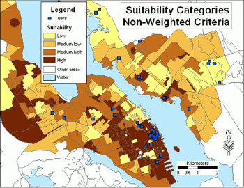
Figure 4.Suitability categories - non-weighted criteria.Click image for larger view.
The suitability using weighted criteria was calculated according to the following simple formula:
Weighted suitability = (0.05 * Ranked Population aged 18 - 40 (%)) +
+ (0.2 * Ranked Average disposable income) +
+ (0.05 * Ranked Households with one person (%)) +
+ (0.2 * Ranked Spending on food in restaurants (%)) +
+ (0.1 * Ranked Spending on alcohol in licensed premises (%)) +
+ (0.05 * Ranked Spending on food between meals (%)) +
+ (0.15 * Ranked Spending on prerecorded music (%)) +
+ (0.2 * Ranked Spending on live staged performances (%))
Figure 5 shows the geographical distribution of suitability categories using weighted criteria.
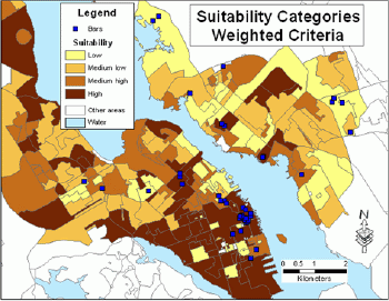
Figure 5.Suitability categories - weighted criteria.Click image for larger view.
Analyze the results and present them to the decision makers
The discussed results represent only one of many possible alternatives. The results have to be checked against reality.This can lead to the modification of initial criteria and/or ranking and weighting schemes. The model has to be adjusted and re-run.More alternative results can be produced.Usually a group of experts is involved in choosing between alternatives.
A cross-tabulation of non-weighted vs.weighted suitability categories
Applying weights to suitability variables altered the original suitability even though the maps (Figures 4 and 5) look somewhat similar.The values on the diagonal in the cross-tabulation table (Table 6) indicate that total agreement between both classifications (considering all categories) was fairly high (67.5%).The agreement was almost 80% for the category 'low', whereas for the category 'medium high' the agreement was much lower (57.6%).Row values indicate how each non-weighted category was re-distributed between weighted categories.Changing weights would produce different results.For example, the weight for the variable Average disposable income could be lowered and the weight for the variable Spending on alcohol in licensed premises (%) could be increased.Again, it is so important that weights are developed by a group of experts, just to narrow down the number of alternative results.
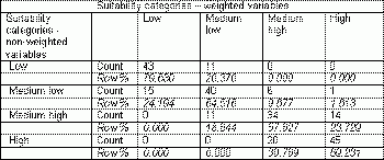
Table 6.A cross-tabulation of non-weighted vs.weighted suitability categories. Click image for larger view.
Weighted suitability categories vs.geodemographic segments
The cross-tabulation of PSYTE clusters and suitability categories brings an interesting insight into the relationship between these two features (Table 7).Clusters from 1 - 60 are ranked on average household income with cluster number 1 being the wealthiest.For example, category 'high' coincides geographically with clusters: 4 - Urban Gentry, 20 - Young Urban Professionals, 36 - Young Urban Intelligentsia, 40 - University Enclaves.Category 'medium high' coincides with some of just mentioned clusters and, additionally, with cluster 51 - Young City Singles and 56 - Urban Bohemia.These clusters form a customer base for various kinds of bars and should be studied further.
The following clusters coincide with 'low' suitability: 59 - Big City Stress, 48 - Struggling Downtowns, 28 - Conservative Homebodies.The 'medium low' category is best represented in areas with cluster 17 - Aging Erudites, 51 - Young City Singles and 33 - High-rise Sunsets.All mentioned clusters should rather be avoided when choosing best areas for a bar.
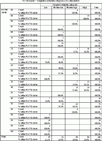
Table 7.Cross-tabulation of PSYTE clusters and weighted suitability categories.Click image for larger view.
Cluster numbers listed in Table 7 have corresponding nicknames: 3 - Suburban Executives, 4 - Urban Gentry, 6 - Mortgaged in Suburbia, 7 - Technocrats and Bureaucrats, 8 - Stable Suburban Families, 16 - Old Bungalow Burbs, 17 - Aging Erudites, 20 - Young Urban Professionals, 27 - Old Towns' New Fringe, 28 - Conservative Homebodies, 29 - Young Urban Mix, 33 - High-rise Sunsets, 35 - Town Renters, 36 - Young Urban Intelligentsia, 40 - University Enclaves, 41 - High-rise Melting Pot, 48 - Struggling Downtowns, 51 - Young City Singles, 56 - Urban Bohemia, 58 - Aged Pensioners, 59 - Big City Stress, 60 - Old Grey Towers, NC - Not Classified.
Distribution of competitors vs.weighted suitability categories
The point in polygon analysis using the spatial join operation allowed for counting quickly the number of competitors in each suitability category.As it can be seen from Table 8, bar owners know pretty well where their best markets are.Of the total number of bars included in this case study, 62.5% is located within primary markets with high suitability (25.67% of the study area).
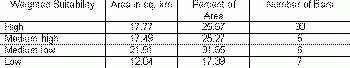
Table 8.Number of existing bars vs.weighted suitability categories. Click image for larger view.
What areas should then be considered as most attractive for locating another bar? The existing bars are concentrated in the downtown of Halifax.As can be seen in Figures 3, 4 and 5, the downtown of Halifax still has a high potential for business expansion.It would depend on additional factors (type of music, type of food, etc.) whether a new bar should be located nearby existing bars or in other highest scoring areas.
Final remarks
The suitability analysis presented in this article is very subjective. However, an attempt was made to make the process more formal by following the main steps of modeling methodology.Suitability modeling produces quantifiable results and identifies the best areas, however, it does not give a final answer to the question 'where?' to locate a business.The highest scoring areas within category 'high' could be considered as the most suitable ones and investigated further using site evaluation techniques supported by trade area analysis.Local demographics, site characteristics, traffic flow patterns, retail structure and many other factors would be considered in the final site selection decision.
References:
Dickey, John, W.1978.Analytic techniques in urban and regional planning: with applications in public administration and affairs; McGraw-Hill
Ghosh, Avijit.McLafferty, Sara, L.1987.Location Strategies for Retail and Service Firms; Lexington Books.
Munroe, S.Nurani, Z.1999.How to Solve Multi-Facility Location Problems.Business Geographics.May, pp.18-20
The analysis of markets can be performed at three spatial levels (Ghosh, McLafferty, 1987).They vary from the regional scale (metropolitan areas, cities, towns, etc.), where areas with the greatest market potential are found, to the local scale in which specific sites for locating new stores are evaluated.
The first level involves the examination of such factors as population size, population projections, demographic and socioeconomic characteristics of the population, income and existing competition. Based on these factors, conclusions can be drawn regarding the market size, structure and saturation.
The second level of market analysis determines the spatial differentiation of market potential within a selected city or metropolitan area.The extent to which demographic and socioeconomic characteristics of the population match the profile of firm's target market is studied at this level, along with such factors as land use/zoning, housing patterns, travel and shopping patterns, transportation networks, etc.The analysis of the competition must also be included at this level, resulting in the list of sub-areas ranked from the point of view of the suitability for a business expansion.
The third level of market analysis is site evaluation.Its objective is to prepare a list of potential sites from which the best site can be chosen.There are various approaches to retail site evaluation, ranging from simple ones such as ranking, to complex ones such as the location-allocation modeling.Each of these approaches involves the idea of key factors - variables essential to a firm's success.GIS can be used at all levels of spatial analysis of markets.
The site evaluation process for the chain, or network of stores or service facilities is much more complex than for an independent facility.This is because the addition of a new store affects the entire network of stores.The evaluation of these impacts requires testing multiple scenarios using such techniques as, for example, location-allocation modeling integrated with GIS.
Another challenge for analyzing a network is to answer the question whether or not to enter a new market or expand in an existing one.Many economic reasons (minimizing per-unit marketing, distribution and management costs, gaining strong market presence) indicate that re-evaluating existing markets is more important than identifying the new ones (Munroe, Nurani, 1999).
This article illustrates how GIS technology, combined with some statistical analysis, can be used for identifying potential markets for the hypothetical business - a live music bar.Two approaches are applied: multiple linear regression and suitability modeling.The target variable that is modeled using the regression is the Expenditure on live staged performances as percentage of spending on spectator entertainment performances.In suitability modeling the target variable becomes one of the most important criteria for the analysis.The analyses presented in this article correspond to the second level of market analysis that includes the study of spatial differentiation of market potential within selected metropolitan area, in this case study, Halifax-Dartmouth, Nova Scotia.
Selecting variables for analysis
In the process of finding potential markets, there is usually an abundance of available data.Potential input variables should be extracted from such data sets as Census, consumer spending categories, and point data sets representing location of competitors or location of other important facilities.Selecting the most suitable and relevant variables for further analysis is time consuming but critical.After preparing a long list of potential variables, some criteria should be applied to shorten the list of candidates for variables that will be used as predictors.
The first criterion is to choose variables that are spatially differentiated.The coefficient of variation, which is the ratio between the standard deviation and arithmetic mean, can be used for this purpose.However, all variables (the initial list included sixteen of them) selected for this case study showed similar level of spatial variation and this criterion alone did not help in eliminating some of them.
The second criterion is to analyze how significant is the correlation between a potential predictor and all target variables.Based on this criterion, two potential predictors were eliminated: the density of population and the sum of distances to universities.All other variables revealed a very significant correlation (at the significance level 0.01) with the target variable.
The next approach was to use a neural network algorithm for showing the relative importance of predictors.Table 1 presents the order of predictors according to their importance determined by the neural network algorithm.The most important predictor is the spending on prerecorded music (%); the least important is the distance to closest bar (competitor).
Table 1.Importance of predictors determined by
the neural network algorithm.
Predicting spending on live staged performances using a regression model
The most common approach to predicting the target variable (Spending on live staged performances) is to apply a multiple linear regression model.The stepwise method was used for entering and removing independent variables from the regression model.This method revealed that the following variables entered the model in the following order:
- Spending on food in restaurants (%)
- Average disposable income
- Spending on alcohol in licensed premises (%)
- Population aged 18 - 40 (%)
- Spending on food between meals (%)
- Spending on prerecorded music (%)
- Households with one person (%).

Figure 1.Strength of predictors. Click image for larger view.
It is expected that all independent variables from the regression model are significantly correlated with the target variable.However, collinearity occurs if these variables are inter-correlated among themselves.The tolerance coefficient can be calculated for each variable and used for measuring the collinearity.This coefficient is calculated as the difference 1- R2, where R is the multiple correlation of a given variable with all other independent variables.If this coefficient is close to zero, a problem with collinearity exists.As demonstrated in Figure 2, the tolerance coefficient differs from zero for all the variables, therefore all of them can be used for determining the market potential.However, spending on food in restaurants and spending on prerecorded music has the strongest correlation with other variables, whereas the percent of population aged 18 - 40 has the weakest correlation.
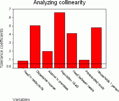
Figure 2.Coefficients of tolerance.Click image for larger view.
The regression model used for predicting the target variable has the form of the following linear equation:
Predicted target variable (Spending on live staged performances %) = -1.735 +
+ 0.155(Spending on food in restaurants %) + 0.00014(Average disposable income) +
+ 0.228(Spending on alcohol in licensed premises %) +
+0.0546(Population aged 18-40 %) - 0.485(Spending on food between meals %) +
+ 0.293(Spending on prerecorded music %) - 0.0467(Households with one person %)
This model is very efficient for prediction, since the correlation between the actual and predicted values is very significant (R = 0.916).Even if actual values are close to predicted, in some areas these residuals (differences) can be significant.If actual values are higher than predicted ones, the market is over-performing and there are some factors that should be found for explaining this phenomenon.If predicted values are higher than actual ones, the market is under-performing and such areas can be considered as untapped market potential.Because residuals are unique for each spatial unit (polygon), they were first standardized and then reclassified into four categories (Table 2).High negative residuals represent untapped market potential good for business.Low negative residuals correspond to moderately good areas for the business expansion.The positive and high positive residuals represent over-performing markets and indicate, respectively, medium low and low market potential (Figure 3).
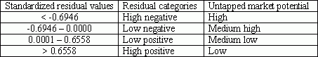
Table 2.Correspondence between residuals and market potential categories. Click image for larger view.
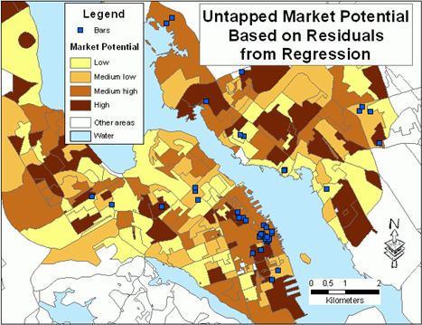
Figure 3.Untapped market potential based on residuals from regression. Click image for larger view.
Analyzing areas with high untapped market potential
In order to perform further analyses, the variables (predictors) were also classified into four categories (low, medium low, medium high and high).Earlier analysis revealed that there is a very significant correlation between each predictor and the target variable.At this point, the question arises: is there a significant association among these variables after they were recoded into four categories? A cross-tabulation was performed for analyzing the association among every predictor and a target variable, each having four categories.The chi-square statistic was used for testing the significance of the association.All associations are significant.Each cross-tabulation resulted in a 4x4 table.The most interesting cell in each 4x4 table is one corresponding to 'high' untapped market potential and category 'high' for each predictor.Table 3 presents the percent of occurrences for each predictor for 'high' / 'high' categories.For example, within the areas representing the high untapped market potential, there are 52.9% occurrences of areas representing high spending on food in restaurants, but only 10.3% of areas with high average disposable income.If the distribution is uniform, the expected value would be 25% (100% spread evenly over four categories).High values for all predictors, except for the disposable income, show higher concentration in areas with high untapped market potential.
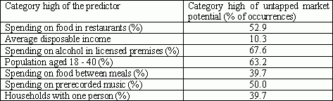
Table 3.Comparison of category 'high' of untapped market potential with category 'high' for all predictors. Click image for larger view.
Untapped market potential vs.geodemographic segments
Identification of geodemographic segments that exist in areas with high untapped market potential can help make business decisions by focusing on such segments.On the other hand, if a given geodemographic segment corresponds mainly to areas with low untapped market potential (high positive residuals), that segment should be avoided when considering a location of a given business.Canadian PSYTE clusters were cross-tabulated with four categories of untapped market potential.In areas with high untapped market potential there are 12 different PSYTE clusters, and six of them can be found only in this category.In areas with a low untapped market potential there are eight PSYTE segments and one of them can be found exclusively in this category.These segments should be avoided.More comments on the relationship between clusters and results of modeling can be found in the section titled "Weighted suitability categories vs.geodemographic segments."
Suitability modeling
Suitability analysis represents one of the most common GIS modeling techniques.Some of the factors that make it so attractive include:
- They aim to find locations that are best suited for a specified activity
- As abstractions of reality, they simplify complex problems for easier understanding
- They provide a logical framework for organizing the criteria for analysis
- They are used to test alternatives
- The modeling results are quantifiable (use measures of suitability)
- They allow for simultaneous evaluation of all studied areas (every area is assigned a suitability score)
- They are easy to comprehend and implement
- They help to make decisions.
The main components of the modeling methodology for determining suitability include the following steps, which will be further discussed below.
1.Define the model
a. Define the problem
b. Select variables for analysis and get the data2.Reclassify data into suitability ranks and develop weights
3.Run the model: combine suitability ranks with suitability weights to calculate the final score
4.Analyze the results and present them to the decision makers
c. Cross-tabulation of non-weighted vs.weighted suitability categories
d. Weighted suitability categories vs.geodemographic segments
e. Distribution of competitors vs.weighted suitability categoriesDefine the problem
The problems for which models are developed can be of various complexities.A team discusses all of the issues associated with the problem being modeled.The complex problem has to be often broken down into smaller problems.Therefore there is usually one general goal and many sub-goals in the model.
In this article, the task is relatively easy to model.The goal is to find the most suitable areas for locating a live music bar.In order to achieve this goal, potential markets will be evaluated using relative suitability scores.Every area included in the analysis will get a suitability score assigned and areas with highest scores will be considered the best ones.
Select variables for analysis and get the data
The selection of criteria for analysis and corresponding data is an integral part of model definition.For this case study, a range of variables describing demographic, socio-economic and lifestyle characteristics of the consumers was selected.Let us assume that a team of experts selected the following variables.
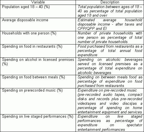
Table 4.Variables for suitability analysis.Click image for larger view.
An ideal customer of the live music bar would then be 18 to 40 years old, a single, with a pretty good income that would allow for certain spending habits listed in Table 4.
Reclassify data into suitability ranks and develop weights
This is the hardest and most subjective part of the modeling methodology.Because the data for the analysis is usually on different measurement scales (nominal, ordinal, interval, ratio), it is impossible to combine data mathematically without placing it on a common scale.Assigning ranks to original data values is a typical solution for bringing data to a 'common denominator.' The original data is converted (reclassified) into new values - suitability ranks -- using experts' judgments.Also weights must be developed to indicate the relative importance of different criteria.Is the age of consumers more important than an average income in the case of locating a live music bar? Assigning ranks and weights is based on preferences. Therefore this step should be completed by a group of experts rather than by a single expert.
One of the group preference assessment techniques is the Delphi method. There is a long tradition in combining the Delphi method with GIS.The purpose of applying this method is to find a group's average preference for assigning ranks and weights.Three characteristics of the Delphi method distinguish it from other preference assessment techniques (Dickey, 1978).
- Anonymity. Each participant anonymously evaluates the rank or weight using a form or questionnaire and submits it to the group facilitator.
- Iteration with controlled feedback. The facilitator analyzes forms, calculates statistics for each rank or weight and produces a summary report for the group.The group reviews the report and each participant has an opportunity to compare his or her own judgment with group's average preference.The group's discussion continues with the focus on the most controversial issues.The participants then vote again, most likely modifying their values based on earlier discussion.In the Delphi sequence each successive submission of a form/questionnaire is referred to as a "round." The group usually reaches consensus in two or three rounds. Consensus is achieved when no assessments cross over (change relative importance) between rounds.
- Statistical response. The Delphi procedure presents a statistical response which includes everyone's opinions.For a single rank or weight the response is usually presented using a mean, a standard deviation (or a median and two quartiles) and others statistics.It is advisable to present the results of each round using a graph or chart.
The assessment of relative importance of different criteria is even more critical than the assignment of ranks.The development of weights should always be a team effort.The weights can be changed to increase or decrease the importance of various suitability criteria.The model can then be re-run to produce alternative results.Weights must add up to 1.For this case study, the following weights were chosen.
Table 5.Weights for suitability criteria.
It was felt that income, spending on food consumed in restaurants, spending on live staged performances and prerecorded music were more important than the other four variables.
Run the model: combine suitability ranks with suitability weights to calculate the final score
The suitability model was run twice: without weights and with weights. In the first case, variables reclassified into five categories were added together to get a cumulative suitability index.This cumulative suitability index was further reclassified into four categories: high, medium high, medium low and low.Figure 4 illustrates spatial differentiation of suitability categories.The map also displays locations of existing bars in the study area.
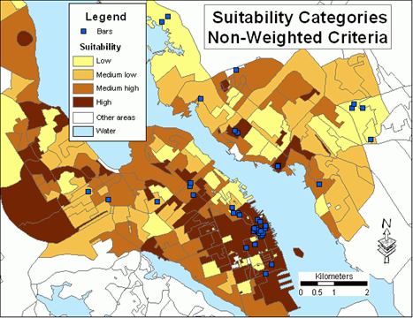
Figure 4.Suitability categories - non-weighted criteria.Click image for larger view.
The suitability using weighted criteria was calculated according to the following simple formula:
Weighted suitability = (0.05 * Ranked Population aged 18 - 40 (%)) +
+ (0.2 * Ranked Average disposable income) +
+ (0.05 * Ranked Households with one person (%)) +
+ (0.2 * Ranked Spending on food in restaurants (%)) +
+ (0.1 * Ranked Spending on alcohol in licensed premises (%)) +
+ (0.05 * Ranked Spending on food between meals (%)) +
+ (0.15 * Ranked Spending on prerecorded music (%)) +
+ (0.2 * Ranked Spending on live staged performances (%))
Figure 5 shows the geographical distribution of suitability categories using weighted criteria.
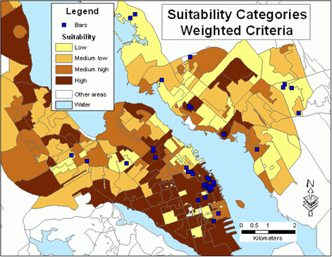
Figure 5.Suitability categories - weighted criteria.Click image for larger view.
Analyze the results and present them to the decision makers
The discussed results represent only one of many possible alternatives. The results have to be checked against reality.This can lead to the modification of initial criteria and/or ranking and weighting schemes. The model has to be adjusted and re-run.More alternative results can be produced.Usually a group of experts is involved in choosing between alternatives.
A cross-tabulation of non-weighted vs.weighted suitability categories
Applying weights to suitability variables altered the original suitability even though the maps (Figures 4 and 5) look somewhat similar.The values on the diagonal in the cross-tabulation table (Table 6) indicate that total agreement between both classifications (considering all categories) was fairly high (67.5%).The agreement was almost 80% for the category 'low', whereas for the category 'medium high' the agreement was much lower (57.6%).Row values indicate how each non-weighted category was re-distributed between weighted categories.Changing weights would produce different results.For example, the weight for the variable Average disposable income could be lowered and the weight for the variable Spending on alcohol in licensed premises (%) could be increased.Again, it is so important that weights are developed by a group of experts, just to narrow down the number of alternative results.

Table 6.A cross-tabulation of non-weighted vs.weighted suitability categories. Click image for larger view.
Weighted suitability categories vs.geodemographic segments
The cross-tabulation of PSYTE clusters and suitability categories brings an interesting insight into the relationship between these two features (Table 7).Clusters from 1 - 60 are ranked on average household income with cluster number 1 being the wealthiest.For example, category 'high' coincides geographically with clusters: 4 - Urban Gentry, 20 - Young Urban Professionals, 36 - Young Urban Intelligentsia, 40 - University Enclaves.Category 'medium high' coincides with some of just mentioned clusters and, additionally, with cluster 51 - Young City Singles and 56 - Urban Bohemia.These clusters form a customer base for various kinds of bars and should be studied further.
The following clusters coincide with 'low' suitability: 59 - Big City Stress, 48 - Struggling Downtowns, 28 - Conservative Homebodies.The 'medium low' category is best represented in areas with cluster 17 - Aging Erudites, 51 - Young City Singles and 33 - High-rise Sunsets.All mentioned clusters should rather be avoided when choosing best areas for a bar.
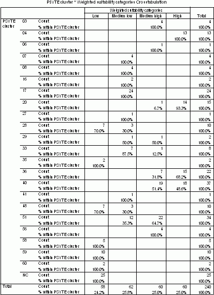
Table 7.Cross-tabulation of PSYTE clusters and weighted suitability categories.Click image for larger view.
Cluster numbers listed in Table 7 have corresponding nicknames: 3 - Suburban Executives, 4 - Urban Gentry, 6 - Mortgaged in Suburbia, 7 - Technocrats and Bureaucrats, 8 - Stable Suburban Families, 16 - Old Bungalow Burbs, 17 - Aging Erudites, 20 - Young Urban Professionals, 27 - Old Towns' New Fringe, 28 - Conservative Homebodies, 29 - Young Urban Mix, 33 - High-rise Sunsets, 35 - Town Renters, 36 - Young Urban Intelligentsia, 40 - University Enclaves, 41 - High-rise Melting Pot, 48 - Struggling Downtowns, 51 - Young City Singles, 56 - Urban Bohemia, 58 - Aged Pensioners, 59 - Big City Stress, 60 - Old Grey Towers, NC - Not Classified.
Distribution of competitors vs.weighted suitability categories
The point in polygon analysis using the spatial join operation allowed for counting quickly the number of competitors in each suitability category.As it can be seen from Table 8, bar owners know pretty well where their best markets are.Of the total number of bars included in this case study, 62.5% is located within primary markets with high suitability (25.67% of the study area).
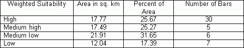
Table 8.Number of existing bars vs.weighted suitability categories. Click image for larger view.
What areas should then be considered as most attractive for locating another bar? The existing bars are concentrated in the downtown of Halifax.As can be seen in Figures 3, 4 and 5, the downtown of Halifax still has a high potential for business expansion.It would depend on additional factors (type of music, type of food, etc.) whether a new bar should be located nearby existing bars or in other highest scoring areas.
Final remarks
The suitability analysis presented in this article is very subjective. However, an attempt was made to make the process more formal by following the main steps of modeling methodology.Suitability modeling produces quantifiable results and identifies the best areas, however, it does not give a final answer to the question 'where?' to locate a business.The highest scoring areas within category 'high' could be considered as the most suitable ones and investigated further using site evaluation techniques supported by trade area analysis.Local demographics, site characteristics, traffic flow patterns, retail structure and many other factors would be considered in the final site selection decision.
References:
Dickey, John, W.1978.Analytic techniques in urban and regional planning: with applications in public administration and affairs; McGraw-Hill
Ghosh, Avijit.McLafferty, Sara, L.1987.Location Strategies for Retail and Service Firms; Lexington Books.
Munroe, S.Nurani, Z.1999.How to Solve Multi-Facility Location Problems.Business Geographics.May, pp.18-20
From Our Homepage
Saying Farewell to an Amazing Journey
Communicating with Maps
Is There a GIS Career Ladder?
What does it mean to be geospatially smart? Series
Ways Real Estate and Property Developers Utilize Melissa GeoData for Data-Driven Decisions
Unlocking Value From Daily Satellite Imagery and Insights
Maximizing the Value of Your Address Data with Geo Addressing
How Indoor Mapping Enhances the Security of Smart Buildings
Look Ahead: AI, Location Intelligence and Efficiency
Collaboration Takes on Sea Level Rise & Dynamic Technology Environments
Brownies for Brownfields
Has Everything Been Mapped Already?
How Is Data Literacy Changing in an Artificial Intelligence Landscape
Portfolios for GIS Professionals: More Than Just Maps
How to Create a Distance Matrix in QGIS - A Step-by-Step Guide
7 Ideas for Bringing GIS into the K-12 Classroom
The Geography of Movement