Anyone who has ever used a map understands that the way in which the information is portrayed on the map can make it easier or harder to use. Imagine if a map of the United States showed every surface road in the country. It would be a mess. The same is true for digital maps rendered on screen. Cartographic skills are needed to make the maps useful to users in the GIS world. Most applications have this part down to a science, so it is rarely a problem and many maps can be easily customized to show the features and layers needed.
Even more important than visualization is the network aspect of the roads associated with the map data. The underlying map data used to route vehicles are an integral part of any vehicle routing application. The map may impact the visualization part of those applications, but it is even more important when it comes to the networking properties of the map data. Why? Because the algorithms, which determine how to assign stops and how to drive to and sequence stops, are completely dependent on the map's network dataset.
Map providers offer attribute data for transportation companies including size and weight restrictions. These restrictions get a lot of press. This article will focus on the core map data and the utilization of those data, because these attributes affect every company using digital maps for routing.
Accuracy of the Road Network
Many factors impact the accuracy of the road network. New roads are built, some existing roads are modified and a very few of them go away. So the timeliness of the data is important.
The age of the network map data can make a big difference, especially if the map data are used for a system that is routing in areas where new housing developments or businesses are popping up. Telephone and utility companies, construction companies, material and appliance delivery companies and others need up-to-date maps for routing. So that begs the question: how often should maps be updated? On the average for most businesses, I would recommend updating the maps at least annually. Road systems change, even in well established areas. Keeping the network up to date is important. Some businesses may need more frequent updates, but you probably won't know how frequent until you start using the maps in your system and problems arise in geocoding and routing. Some businesses require semi-annual, quarterly and even monthly updates.
No matter how often the map is updated, the digital map will never be completely accurate. The map companies have update cycles and procedures they must follow. Errors are found and new roads built, so updates are coming in to them daily. They compile the inputs, analyze and verify them, and then make updates to their databases. This takes time. Some large corporations actually edit their own data to reflect changes in roads, but this is not the norm. Only businesses such as the larger delivery companies need, and can afford, to do this sort of map editing on their own; the average company relies on the data that map providers sell.
Network Connectivity and Road Speeds
Connectivity is important. To digitally travel to your stops along the map network, the geocoded locations first must snap to the nearest points on the network in order for the routing application to assign and schedule stops. To understand how this all works, let's begin with a common example: an Internet service that provides driving directions.
When you use a typical, free Internet service to get driving directions, the application usually asks if you want the shortest path or the quickest path. Sometimes it asks if you prefer to use or avoid highways. The reason for this is simple. It impacts how you get from one point to another.
Each segment of road in the network dataset has an associated distance and road speed stored with it. The sum of all the distances assigned to each segment of road between two points constitutes the distance between those points, as specified by the distance data for each road segment. Likewise, the sum of the ratio of the distance and road speed assigned to each segment of road between two points constitutes the travel time between those points, provided by both the distance and speed data for each road segment.
The diagram below is a simplified example. We have two points, A and B, with five road segments shown between them.
Assume each segment has the following properties:
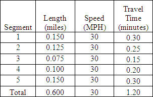 |
The distance between the points is 0.6 miles when you sum up the length value of each of the five segments. Similarly, the time to traverse the distance is 1.2 minutes based on the 30 mph speed factor assigned to each segment. The distance is obviously traversed at an average speed of 30 mph.
 |
It gets a little more complicated when different road segments have different assigned speeds. For example:
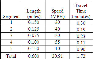 |
The time it takes to travel the 0.6 miles from A to B now changes based on the time to traverse each segment and the road speed assigned to it. So now, with each segment's new assigned road speed, it should take 1.72 minutes to travel from A to B.
While calculating the travel time along a known path is easy to visualize, deciding what path to take between A and B is a little more challenging. Let's make the path between A and B a simple set of points a few blocks apart in an urban environment. It might look like this:
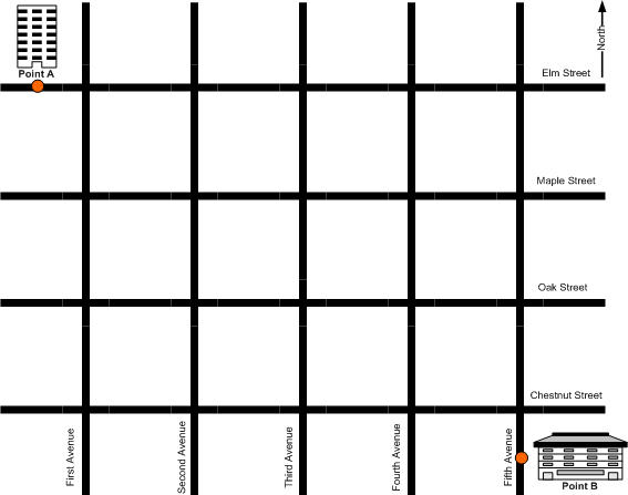 |
Just on the nine streets shown above, a number of paths are available between points A and B. Going east on Elm to First Avenue, you can continue straight or turn. The same sort of choice occurs at the next intersection. Without going out of this small network of roads (assuming there are roads connected outside of this that could also somehow be traversed), there are dozens of ways to go from A to B. Since there is a grid arrangement of equal length streets, the shortest distance in this example occurs 15 different ways from A to B. To find the shortest travel time, you have to apply a speed factor to each road segment. If they are all the same, the system chooses one of the 15 paths based on some criteria. If they vary, the system weighs how long it takes to traverse each segment, as it did in the simple example, and comes up with the shortest travel time.
Hierarchical Routing
If there are equal choices to be made (same distance or same time), a preference for some roads over others can be made via some sort of hierarchy in the road network or some predefined rules in the network database. Programmers do this in cases where things are equal because the program has to make some decision, and these predefined rules attempt to improve routing performance. In cases where there are large numbers of possibilities, the system tries to limit the number of possible paths taken into the calculation. Even with this little example, you can imagine all the additional city roads outside of our grid that are also connected and would allow passage from A to B. Without some common sense rules, the system might take all day just to figure this out.
Hierarchical routing is a concept that bears discussion. You might have heard that term used in reference to how some network datasets do routing calculations. Let's say you want to go from New York to Los Angeles. There are many roads you could take, but logically you want to hop on a nearby road with the highest speed limit that takes you to the interstate highway system. Once on the interstate highways, you stay on them until you reach somewhere near your destination. To emulate this and to simplify finding a path between New York and Los Angeles, a hierarchical routing approach would find the fastest (or shortest) way to the interstate highways from your starting location in New York and ending location in Los Angeles. It would only use the interstate highways to pick roads which are the fastest (or shortest) to travel between the highway entry and exit locations. This concept is great when you are doing long distance routing and works in many short distance applications, as well.
There are a few times when the hierarchical routing system does not benefit users. In some instances drivers may not favor highway travel. Drivers often avoid highways in urban areas because of traffic conditions such as volume and accidents. A beer delivery driver may not want to suffer the consequences of getting stuck on an interstate in Chicago or Dallas when he has only a relatively short distance between some or all stops. In cases like this, hierarchical routing is not good because it does not model how drivers actually drive their vehicles. The system will select a highway if it makes sense, but not simply because the hierarchical routing scheme says to do so.
Road Classifications
The nature of routing and path finding on map network datasets usually revolves around shortest times. Estimating the shortest time between points requires the network dataset to have speed attributes that resemble the driving conditions. Map providers such as NAVTEQ and Tele Atlas assign default road speeds to each road segment based on the type of road. The U.S. Census Bureau defines these road types in its TIGER (Topologically Integrated Geographic Encoding and Referencing) database of selected roads. This is an extensive database and it is the basis of the products sold by map vendors such as NAVTEQ and Tele Atlas. They add a lot of quality to the Census Bureau's TIGER maps. The free TIGER data can be used to route and geocode. The results tend to be poor, however, if TIGER data are the basis for an application for address matching or road network quality. There is value in being able to geocode and route accurately, and that is what the mapping companies provide for their users.
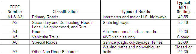
Roads are classified by census feature class codes (CFCC). These road features are classified with the letter A and a number depending on the type of the road. Other non- road features are also classified in this system but are not used for routing vehicles. These classes are:
Primary Highway With Limited Access. Interstate highways and some toll highways are in this category (A1) and are distinguished by the presence of interchanges.
- Primary Road Without Limited Access. This category (A2) includes nationally and regionally important highways that do not have limited access as required by category A1. It consists mainly of U.S. highways, but may include some state highways and county highways that connect cities and larger towns. A road in this category must be hard-surface (concrete or asphalt). It has intersections with other roads, may be divided or undivided, and may have multi-lane or single-lane characteristics.
- Secondary and Connecting Road. This category (A3) includes mostly state highways, but may include some county highways that connect smaller towns, subdivisions and neighborhoods. The roads in this category generally are smaller than roads in category A2, must be hard- surface (concrete or asphalt), and are usually undivided with single-lane characteristics. These roads usually have a local name along with a route number and intersect with many other roads and driveways.
- Local, Neighborhood and Rural Road. A road in this category (A4) is used for local traffic and usually has a single lane of traffic in each direction. In an urban area, this is a neighborhood road or street that is not a thoroughfare belonging in categories A2 or A3. In a rural area, this is a short-distance road connecting the smallest towns; the road may or may not have a state or county route number. Scenic park roads, unimproved or unpaved roads, and industrial roads are included in this category. Most roads in the nation are classified as A4 roads.
- Vehicular Trail. A road in this category (A5) is usable only by four-wheel-drive vehicles, is usually a one-lane dirt trail, and is found almost exclusively in very rural areas. Sometimes the road is called a fire road or logging road and may include an abandoned railroad grade where the tracks have been removed. Minor, unpaved roads usable by ordinary cars and trucks belong in category A4, not A5.
- Road with Special Characteristics. This category (A6) includes roads, portions of a road, intersections of a road, or the ends of a road that are parts of the vehicular highway system and have separately identifiable characteristics.
- Road as Other Thoroughfare. A road in this category (A7) is not part of the vehicular highway system. It is used by bicyclists or pedestrians, and is typically inaccessible to mainstream motor traffic except for private-owner and service vehicles. This category includes foot and hiking trails located on park and forest land, as well as stairs or walkways that follow a road right-of-way and have names similar to road names.
There are also sub-classifications for each classification of road. For example, an A11 sub-classification is a primary road with limited access or interstate highway, unseparated. An A25 is a primary road without limited access, U.S. highways, separated. An A33 is a secondary and connecting road, state highways, unseparated, underpassing. An A42 is a local, neighborhood and rural road, city street, unseparated, in tunnel. An A51 is a vehicular trail, road passable only by 4WD vehicle, unseparated. An A65 is a ferry crossing, the representation of a route over water that connects roads on opposite shores, used by ships carrying automobiles or people. An A73 is an alley, road for service vehicles, usually unnamed, located at the rear of buildings and property.
The major map vendors typically assign the same road speed to each road within each class in their products unless the buyer asks for some other customization. These settings can be customized to classes and sub-classes or regionally if specified, depending on the type of product. Typical settings you will see in various applications for each classification are:
 |
Many routing applications allow the user to modify these settings for road classifications. For example, the Esri product, ArcLogistics Route, allows the user to set these speeds by road class nationwide in its SDC dataset (or any dataset the user installs with ArcLogistics).
Ed. Note: Read part two of this article that addresses speeds, impedances, and live and historic traffic data .