This article looks at the next step in LBS development
- creating a mobility profile for a mobile user to model where that
user is likely to be at specific times on different days of the week.
We leave you to imagine what the killer app for such a capability would
be. This article describes what’s coming, and some of the technical
challenges being addressed.
Within the last few years, there has been a massive surge of interest in wireless positioning methods and applications using wireless positioning information. The main reasons for this surge are:
LBS services can broadly be classified as emergency services, tracking services and entertainment services. Some services may require almost an exact position, whereas others can be built on less accurate locations such as cell segment, cell or even location area (several cells) information. However, all such services are based on points (exact locations) and areas (cell or location areas, city or even country).
There is yet another basis for location services - the exact trajectory (mobility profile) of a mobile user. There is a plethora of services that could be based on a mobility profile. Mobility models studied so far and used in location management (IS-41) can do very little to develop a mobility model for each individual user. The best way is to use individual users’ mobility traces.
From the mobility perspective, you can categorize mobile users into three categories: unpredictable users, partially predictable users and predictable users. The majority of the users will fall into the last two categories. The LBS industry needs to focus on the predictable users, which are quite a large portion of the mobile community. Such users can be associated with a trajectory, a spatiotemporal distribution, per day of the week. In a typical mobility model, the mobile activity varies for each day of the week, but remains the same for the same days of the week. If a user has a similar mobility trajectory for two or more days of the same week, it is a special case of the mobility model.
Future Location-based Services (FLBS)
Mobility profiling will give birth to a new class of LBS services, which we will refer to as “future location-based services (FLBS). These services make use of the user’s trajectory on a given day and estimate where the user is likely to be on that trajectory in the future. Here’s a comparison between LBS and FLBS. First, LBS. You are passing by the Sears department store and you receive a soft discount coupon on your phone from the store to come in and buy a shirt to match the jacket you bought some time ago. However, with FLBS, the same offer could be extended well in advance - you get the soft coupon when you are starting on the path to Sears, or even when you are still at home. The FLBS coupon could even be from a Sears competitor located in the same area. What are the killer applications for FLBS? We leave that to your imagination.
The most attractive characteristic of FLBS (over LBS) and mobility profiling is that it uses a lot fewer air resources. A cellular-based location used for LBS uses existing transceivers, communication bandwidth, two-way messaging and a well established infrastructure. Mobility profiling cuts the usage of these air resources, which LBS uses extensively.
To establish a mobility profile for a mobile user, you need to connect all the estimated location points. Each location point is time stamped. The mobile user is profiled for a week. So each day would yield a trace of positions and time stamps. To estimate the mobile traces to get at a mobility profile, you will come across two challenges: the error associated with the location, and the number of such location points available, or polling frequency. We briefly touch on these two issues in the following sections.
Location Estimation Error
There are several technologies for mobile location estimation. Most methods in use now are time-based. Components include time of arrival (TOA), time difference of arrival (TDOA), enhanced observed time difference (E-OTD) and time advance (TA). The location is estimated based on radio frequency signal travel time. All technologies are based on knowing where existing reference points are, such as cellular radio base stations, and then relating them using propagation time from one end (base station) to the other (mobile station). Triangulation is one of the examples.
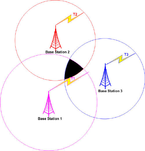
Since the propagating signals travel at the speed of light, anomalies such as interference and reflection due to non-line of sight cause significant errors in calculating time of travel (see figure 1). For perfect triangulation, the three circles shown in figure 1 would intersect at one point, the exact location of the mobile user. However, that’s not the case. Instead we get a region (shaded area) in which the mobile user can be found.
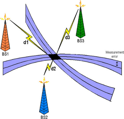
Similarly, with TDOA, instead of getting an exact point, the intersection of two hyperbolas, with time difference of arrival d1,d2 or d2,d3 or d1,d3 from base stations BS1, BS2 and BS3, we also get a black shaded region, as shown in figure 2. So each estimated location is exposed to an error proportional to the size of the shaded area.
Figure 3 depicts the error in location estimation on a road map. The estimated location is associated with an area of error shown here with a circle. The circle corresponds to the shaded areas in figures 1 and 2. The location is corrected using map matching as described below. In a metropolitan area, the error could range from 150 to 500 meters. In rural areas, this could be as much as a few kilometers, because of the large cell size.
Polling Frequency
The second issue is the location polling frequency. Very frequent polling would yield a good spatial distribution - the actual track, obviously offset with error as discussed above. However, creating the actual track would overburden air channels and the location servers. On the other hand, a very low polling frequency would not generate a meaningful trajectory; it would be very ambiguous and erroneous. How frequently you need to find the locations to form a track depends on the speed and direction of the mobile user. If directions change frequently, you need more points to form a trajectory. So we need to poll for location estimation just often enough to yield the information needed to model a trajectory using information and constrains from a GIS database for map matching.
Map Matching
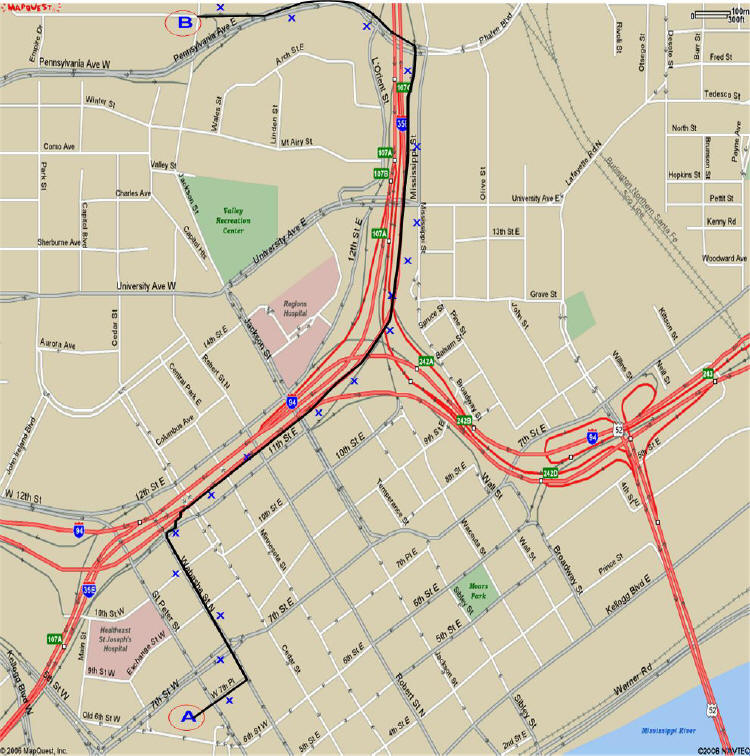
To correct erroneous location coordinates and to fill in between the estimated location points, a technique called map matching is used. It’s also referred to as “snapping.” Because mobile users mostly travel on roads, we can correct the raw location mapping by putting the user on a road. The roads, and related information such as maximum speed, direction and permissible turns, are coded in a GIS database. In this case, you start from a known position such as a home location and build the trajectory with the upcoming points. You use the information from the GIS database and apply it as constraints to help determine the location of the user. The GIS provides all the required geometry and constraints. Below is an example for a mobile user in the Twin Cities in Minnesota. (Please note we have avoided technical details in this example.) Figure 4 shows the points collected for the user, and figure 5 shows the user’s modeled trajectory with a black line.
The mobile user starts from his home, marked location A on the map, and travels toward point B. Between point A and point B, 18 erroneous location positions with time stamps are marked with blue X’s. The first location after point A is map matched to the correct road from the information of the previous point (point A) and the next point, the second X from point A on the map. Similarly the true position of the second point is determined from the exact position of the first point and the direction of the third point. We called this process point tucking. In this case, almost all the candidate streets are one-way roads, so just the direction constraint along with speed information maps the erroneous location point to a true position on the road. Mapping all the points to their true positions and connecting the mapped points generates an estimated path (the black line) shown in figure 5. This travel is one leg of the whole day’s journey. Similarly, we repeat this process for the rest of the legs of travel. This gives us the trace of a mobile user for a whole day, on which a variety of services could be based.
Within the last few years, there has been a massive surge of interest in wireless positioning methods and applications using wireless positioning information. The main reasons for this surge are:
- the fact that new wireless positioning technologies have the capability of alleviating the shortcomings of GPS, such as high power consumption and slow initial position acquisition; and
- legislation in the United States that requires cellular phone operators to provide location information to 911 call centers.
LBS services can broadly be classified as emergency services, tracking services and entertainment services. Some services may require almost an exact position, whereas others can be built on less accurate locations such as cell segment, cell or even location area (several cells) information. However, all such services are based on points (exact locations) and areas (cell or location areas, city or even country).
There is yet another basis for location services - the exact trajectory (mobility profile) of a mobile user. There is a plethora of services that could be based on a mobility profile. Mobility models studied so far and used in location management (IS-41) can do very little to develop a mobility model for each individual user. The best way is to use individual users’ mobility traces.
From the mobility perspective, you can categorize mobile users into three categories: unpredictable users, partially predictable users and predictable users. The majority of the users will fall into the last two categories. The LBS industry needs to focus on the predictable users, which are quite a large portion of the mobile community. Such users can be associated with a trajectory, a spatiotemporal distribution, per day of the week. In a typical mobility model, the mobile activity varies for each day of the week, but remains the same for the same days of the week. If a user has a similar mobility trajectory for two or more days of the same week, it is a special case of the mobility model.
Future Location-based Services (FLBS)
Mobility profiling will give birth to a new class of LBS services, which we will refer to as “future location-based services (FLBS). These services make use of the user’s trajectory on a given day and estimate where the user is likely to be on that trajectory in the future. Here’s a comparison between LBS and FLBS. First, LBS. You are passing by the Sears department store and you receive a soft discount coupon on your phone from the store to come in and buy a shirt to match the jacket you bought some time ago. However, with FLBS, the same offer could be extended well in advance - you get the soft coupon when you are starting on the path to Sears, or even when you are still at home. The FLBS coupon could even be from a Sears competitor located in the same area. What are the killer applications for FLBS? We leave that to your imagination.
The most attractive characteristic of FLBS (over LBS) and mobility profiling is that it uses a lot fewer air resources. A cellular-based location used for LBS uses existing transceivers, communication bandwidth, two-way messaging and a well established infrastructure. Mobility profiling cuts the usage of these air resources, which LBS uses extensively.
To establish a mobility profile for a mobile user, you need to connect all the estimated location points. Each location point is time stamped. The mobile user is profiled for a week. So each day would yield a trace of positions and time stamps. To estimate the mobile traces to get at a mobility profile, you will come across two challenges: the error associated with the location, and the number of such location points available, or polling frequency. We briefly touch on these two issues in the following sections.
Location Estimation Error
There are several technologies for mobile location estimation. Most methods in use now are time-based. Components include time of arrival (TOA), time difference of arrival (TDOA), enhanced observed time difference (E-OTD) and time advance (TA). The location is estimated based on radio frequency signal travel time. All technologies are based on knowing where existing reference points are, such as cellular radio base stations, and then relating them using propagation time from one end (base station) to the other (mobile station). Triangulation is one of the examples.
Since the propagating signals travel at the speed of light, anomalies such as interference and reflection due to non-line of sight cause significant errors in calculating time of travel (see figure 1). For perfect triangulation, the three circles shown in figure 1 would intersect at one point, the exact location of the mobile user. However, that’s not the case. Instead we get a region (shaded area) in which the mobile user can be found.
 |
Similarly, with TDOA, instead of getting an exact point, the intersection of two hyperbolas, with time difference of arrival d1,d2 or d2,d3 or d1,d3 from base stations BS1, BS2 and BS3, we also get a black shaded region, as shown in figure 2. So each estimated location is exposed to an error proportional to the size of the shaded area.
 |
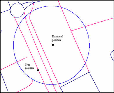 |
Figure 3 depicts the error in location estimation on a road map. The estimated location is associated with an area of error shown here with a circle. The circle corresponds to the shaded areas in figures 1 and 2. The location is corrected using map matching as described below. In a metropolitan area, the error could range from 150 to 500 meters. In rural areas, this could be as much as a few kilometers, because of the large cell size.
Polling Frequency
The second issue is the location polling frequency. Very frequent polling would yield a good spatial distribution - the actual track, obviously offset with error as discussed above. However, creating the actual track would overburden air channels and the location servers. On the other hand, a very low polling frequency would not generate a meaningful trajectory; it would be very ambiguous and erroneous. How frequently you need to find the locations to form a track depends on the speed and direction of the mobile user. If directions change frequently, you need more points to form a trajectory. So we need to poll for location estimation just often enough to yield the information needed to model a trajectory using information and constrains from a GIS database for map matching.
Map Matching
To correct erroneous location coordinates and to fill in between the estimated location points, a technique called map matching is used. It’s also referred to as “snapping.” Because mobile users mostly travel on roads, we can correct the raw location mapping by putting the user on a road. The roads, and related information such as maximum speed, direction and permissible turns, are coded in a GIS database. In this case, you start from a known position such as a home location and build the trajectory with the upcoming points. You use the information from the GIS database and apply it as constraints to help determine the location of the user. The GIS provides all the required geometry and constraints. Below is an example for a mobile user in the Twin Cities in Minnesota. (Please note we have avoided technical details in this example.) Figure 4 shows the points collected for the user, and figure 5 shows the user’s modeled trajectory with a black line.
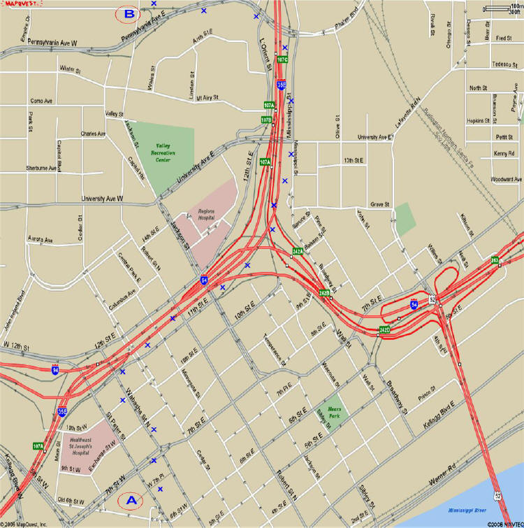 |
The mobile user starts from his home, marked location A on the map, and travels toward point B. Between point A and point B, 18 erroneous location positions with time stamps are marked with blue X’s. The first location after point A is map matched to the correct road from the information of the previous point (point A) and the next point, the second X from point A on the map. Similarly the true position of the second point is determined from the exact position of the first point and the direction of the third point. We called this process point tucking. In this case, almost all the candidate streets are one-way roads, so just the direction constraint along with speed information maps the erroneous location point to a true position on the road. Mapping all the points to their true positions and connecting the mapped points generates an estimated path (the black line) shown in figure 5. This travel is one leg of the whole day’s journey. Similarly, we repeat this process for the rest of the legs of travel. This gives us the trace of a mobile user for a whole day, on which a variety of services could be based.
 |
From Our Homepage
Saying Farewell to an Amazing Journey
Communicating with Maps
Is There a GIS Career Ladder?
What does it mean to be geospatially smart? Series
Ways Real Estate and Property Developers Utilize Melissa GeoData for Data-Driven Decisions
Unlocking Value From Daily Satellite Imagery and Insights
Maximizing the Value of Your Address Data with Geo Addressing
How Indoor Mapping Enhances the Security of Smart Buildings
Look Ahead: AI, Location Intelligence and Efficiency
Collaboration Takes on Sea Level Rise & Dynamic Technology Environments
Brownies for Brownfields
Has Everything Been Mapped Already?
How Is Data Literacy Changing in an Artificial Intelligence Landscape
Portfolios for GIS Professionals: More Than Just Maps
How to Create a Distance Matrix in QGIS - A Step-by-Step Guide
7 Ideas for Bringing GIS into the K-12 Classroom
The Geography of Movement