Author's note: I wrote this
article as a contractor for TCI Software.
The State of Geodata
GIS data holds lots of expectations for users. The data sets are supposed to enable pretty maps with straight lines and smooth curves. They are supposed to be small and compact for easy storage and sharing. And, they are supposed to be accurate in representing what's on the ground.
Those are lofty and sometimes incompatible goals. For years those developing GIS and other types of representational software have tried to balance those demands with others, including the speed of processing. One of the choices some software developers made was not to store curved geometry in mathematical formulae, but rather as "stroked" arcs. Stroking refers to representing curves with many short, straight segments. This storage format sped up some types of calculations. As a result of this decision, there's quite a lot of mapping data in use today in a variety of formats that include stroked arcs. These data sets can be the cause of poor aesthetics in print and online maps (including sharp points and jagged lines), large files (in some cases hundreds of percent larger) and representations that do not match curves in the real world (such as highways and streams).
The good news is that data formats and software products are maturing. Today more software products than ever can analyze datasets in formats that store mathematical curves. What software products and what formats? Most CAD formats have been able to store and use mathematical arcs since they were introduced, as far back as the 1980s. AutoCAD, MicroStation (and many of the GIS products built on them) and other CAD packages store and manipulate entities using curves. Oracle Spatial stores curves, so, too, do Intergraph's GeoMedia Warehouses (Access/SQL Server), Autodesk's MapGuide's SDF3 and GeoConcept's native format. ESRI has updated its key storage format, the geodatabase, to support mathematical curves as well.
This is great news for users of these packages as they create new datasets because they can store data directly in these compact data formats. These formats also provide an opportunity to optimize stroked curves in legacy data. Optimize? That's right, this is the time to make the best choices about how to turn those stroked lines, which may represent linear features or be part of complex polygons, into mathematical curves that meet data user needs. How? By using the new Curvefitter extension to Safe Software's FME 2007.
TCI Software developed Curvefit 15 years ago as an AutoCAD add-on to address the "stroking" challenge, primarily encountered when legacy data was imported. When Safe Software completed the move to what it terms Rich Geometry, which includes support for mathematical curves in FME 2007, it was time to port Curvefit into the Curvefitter extension to FME. The extension adds a new Curvefitter Transformer to the product's long list of transformers.
There is one caveat in using Curvefitter worth noting before going any further: there's no advantage to optimizing geodata with curves if their ultimate destination is a format that can't store curves! (Shapefiles are one example.) But for nearly all other stroked datasets, there will be benefits to Curvefitter data optimization that can be measured aesthetically, in size and in accuracy.
How Curvefitter Works
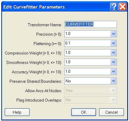
Simply put, Curvefitter examines long lines made up of many segments, called polylines in AutoCAD and other names, including linestrings, in other programs, and determines a "best" combination of curved and straight segments to represent them. To do that, the software takes into account three key goals: compression (how important is file size reduction?), smoothness (how important is overall smoothness of the line?) and accuracy (how important is it for the output to match the input?). Casual users can use default settings and Curvefitter's built-in fuzzy logic will balance the three. Those who need more control for a specific goal can set parameters one at a time, giving each one a different weight (Figure 1).
The user also sets two parameters that control the nature of the output lines and curves. Precision is the most important and defines how far an existing vertex in the dataset can be from the linework in the output dataset. Keep the value small (in units of the data) and the resulting line will follow the existing vertices closely. Make the value larger and the resulting line will be allowed to run above or below the final polyline, up to the amount specified in precision. Flattening determines when relatively flat curves are replaced with straight lines. A curve with a mid-ordinate (a measure of curvature) below this value will be turned into a straight line.
Putting Curvefitter Through its Paces
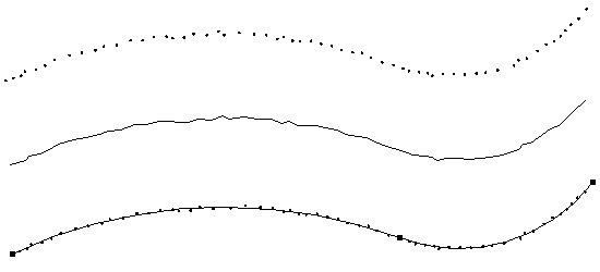
In the figure below, the line in the middle is defined by 59 vertices (shown on top). If you counted, you'd find that 57 short segments make up the line. Curvefitter optimized the line by representing it using just three vertices, that is, just two curved segments (bottom). The black squares show their start and end points. You'll note that the resultant line closely, but not exactly, follows the centers of the vertices.
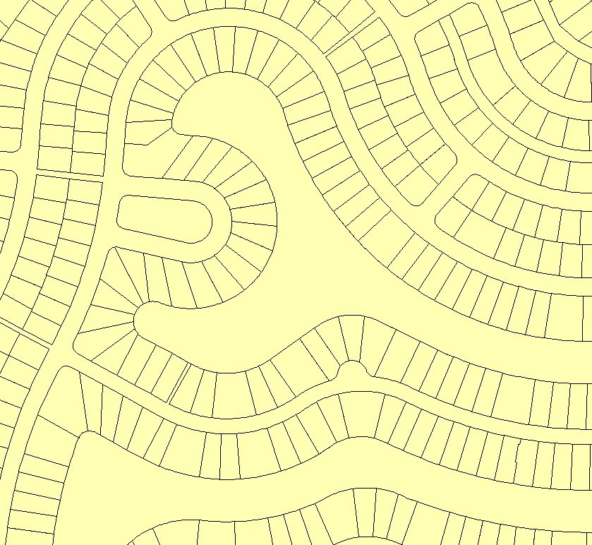
The real power comes when Curvefitter tackles large "real life"-sized datasets. Let's start with some parcel data. Grays Harbor County in Washington State offers its data for free on the Internet (and provided permission to use it for this article). A subset 6.1 MB shapefile was extracted (Figure 4a). That was converted into a DWG file (3.8 MB), MapGuide SDF (4.5 MB), ESRI personal geodatabase (5.4 MB) and file geodatabase (available in ArcGIS 9.2, 1.89 MB) using Safe's Feature Manipulation Engine (FME) core tools.
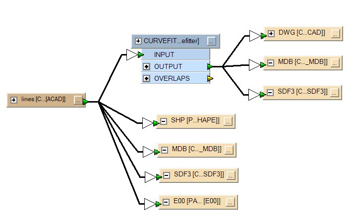
The next step was to run Curvefitter. FME and non-FME users can tease out the process in this FME workspace (Figure 3). A workspace allows FME users to create, edit and save such procedures either to run in the future or imbed in other workspaces.
The Curvefitter precision parameter for this example was set very high, at 0.1, which in this case means 0.1 feet. (The value is always in the native units of the data.) In English, that means that each newly created vertex can be no more than 1/10 of a foot from the original line it represents. Said another way, the vertices are on a tight leash and must stay "very close" to the original linework.
It's also worth noting that Curvefitter can take advantage of existing FME tools to maintain shared boundaries (or not) after optimization depending on user need. For parcels and other data sets with adjacent polygons, it's most likely that users will want shared boundaries to be maintained.
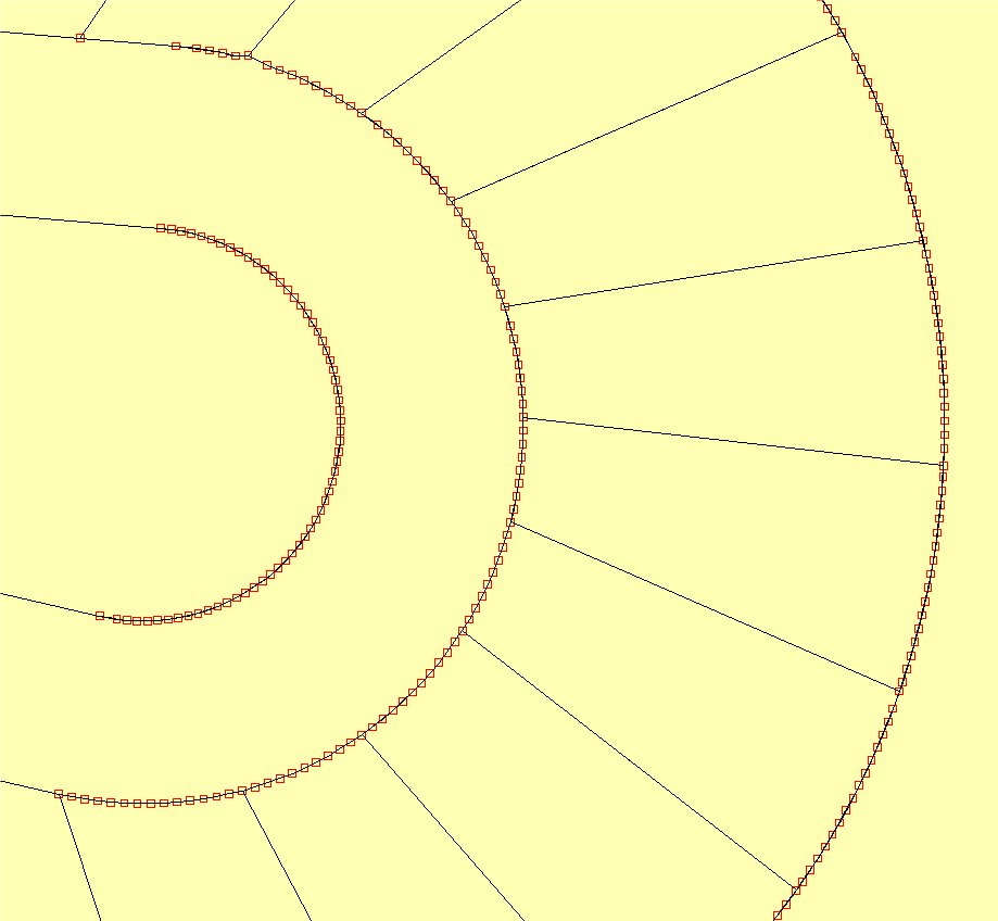
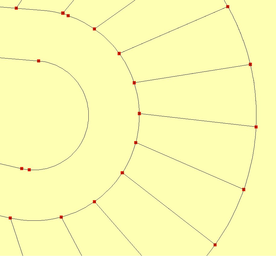
Zooming in on the original data (Figure 3b) you can see there are many, many vertices making up the curved sides of the parcels. After running Curvefitter (Figure 3c), each parcel's curved sides are saved as single arcs, with a few exceptions.
What does that mean for file statistics? The AutoCAD DWG shrank 137% to 1.6 MB. The SDF3 file shrank 181% to 1.6 MB. The ESRI personal geodatabase shrank 12.5% to 4.8 MB. ESRI's new ArcGIS 9.2 file geodatabase shrank 77.5% to 1.09 MB.
The reduction is calculated by using the following formula: % reduction=[Original Size - New Size] / New Size X 100. Or in English, the value is the ratio between what was removed to what is left x 100. A 300% reduction means three parts removed, to one part left, or the resulting file is to 1/4 of the size of the original. A 200% reduction would be two parts removed for one part left; the resulting file is 1/3 the size of the original. Table 1 includes all of the "before and after" values from each example in this article.
From a visual standpoint the curves in the output datasets will remain
curves, no matter how much the viewer "zooms in." Further, when the
parcel map is printed on paper, the parcel's curved edges will appear
smooth.
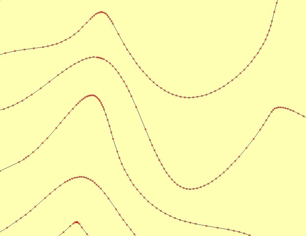
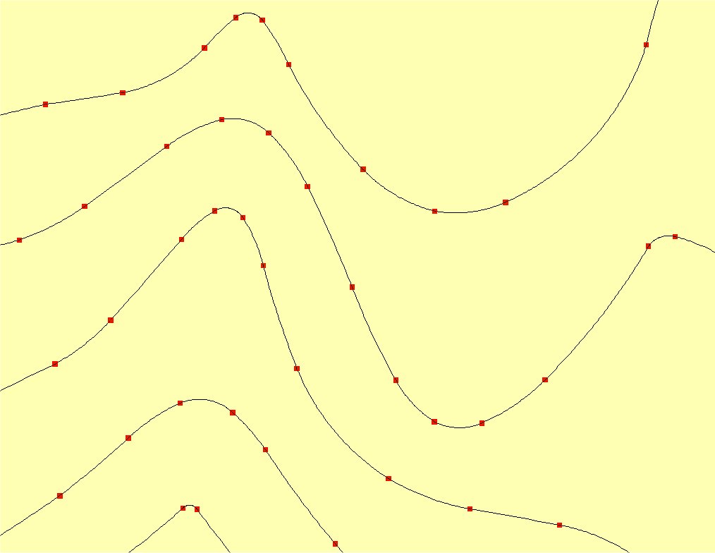
Contour lines create notoriously large CAD and GIS files. Depending on their source, they can also have odd "spikes" and "points" that rarely reflect the real world's topography. See, for example, the bottom-most contour in Figure 4a. This contour line data set originated as a 35.9 MB DWG which spawned, using FME, a 50.8 MB SDF3, a 126.7 MB E00 file, a 56.4 MB personal geodatabase, and a 17.3 MB file geodatabase. After Curvefitter processing (Figure 4b), the DWG dropped 360% to 7.8 MB, SDF3 260% to 14.0 MB, and the personal geodatabase 139% to 23.6 MB. The file geodatabase shrank 65% to 10.5MB. In this case a more moderate precision of 1.0 foot was used, allowing the final vertices to stray up to a full foot from the original linework.
Other large datasets GIS professionals work with are regional or
countrywide geology maps. These define the areas of different types of
surface or subsurface formations and often have many complexly
organized polygons that are ultimately rendered in multicolor thematic
maps. The Natural Resources Canada website
makes datasets for the
country publicly available for download. FME processed the 46.3 MB
shapefile (Figure 5a) to create a 28.5 MB DWG, a 47.8 MB SDF3, a 59.6
MB ESRI personal geodatabase and a 43 MB file geodatabase. Here the
parameters were adjusted to focus on smoothness and accuracy, and
precision was dropped to 20 feet. The AutoCAD file dropped by 391% to
5.8 MB, the SDF3 265% to 13.1, the personal geodatabase 242% to 17.4
and the file geodatabase 378% to 9.0 MB. The integrity of the many
short segments in the original data (Figure 5b) was maintained, as was
the topology, in the Curvefitter output (Figure 5c).
Timing is Everything
Curvefitter comes at the right time for those involved with geospatial data. In the early days of GIS, data collection was the key focus. Today data are abundant, though they bear the legacy of being "well processed." Many of these datasets can be optimized, trimmed down and smoothed out, and as a result become more accurate. Once that's complete, they can be stored in a variety of geospatial data formats that support geometric curves, something not widely available in the past two decades.
It's worth noting from these examples that optimizing shapefiles into ESRI's new file geodatabase yielded impressive results: size reductions on the order of 6:1 using Curvefitter. Further, of all the formats tested, the file geodatabase is the most efficient in terms of file size. (There are other benefits of this format including a 1 TB size limit and cross operating system support.) No matter what the format, smaller optimized files will most definitely play a key role in today's new world of data sharing. Smaller GIS data files, whether purchased online, downloaded free from governments, or sent to mobile devices are far easier to distribute than larger ones. Curvefitter may be the best thing to come along in geospatial data optimization in a long time.
The State of Geodata
GIS data holds lots of expectations for users. The data sets are supposed to enable pretty maps with straight lines and smooth curves. They are supposed to be small and compact for easy storage and sharing. And, they are supposed to be accurate in representing what's on the ground.
Those are lofty and sometimes incompatible goals. For years those developing GIS and other types of representational software have tried to balance those demands with others, including the speed of processing. One of the choices some software developers made was not to store curved geometry in mathematical formulae, but rather as "stroked" arcs. Stroking refers to representing curves with many short, straight segments. This storage format sped up some types of calculations. As a result of this decision, there's quite a lot of mapping data in use today in a variety of formats that include stroked arcs. These data sets can be the cause of poor aesthetics in print and online maps (including sharp points and jagged lines), large files (in some cases hundreds of percent larger) and representations that do not match curves in the real world (such as highways and streams).
The good news is that data formats and software products are maturing. Today more software products than ever can analyze datasets in formats that store mathematical curves. What software products and what formats? Most CAD formats have been able to store and use mathematical arcs since they were introduced, as far back as the 1980s. AutoCAD, MicroStation (and many of the GIS products built on them) and other CAD packages store and manipulate entities using curves. Oracle Spatial stores curves, so, too, do Intergraph's GeoMedia Warehouses (Access/SQL Server), Autodesk's MapGuide's SDF3 and GeoConcept's native format. ESRI has updated its key storage format, the geodatabase, to support mathematical curves as well.
This is great news for users of these packages as they create new datasets because they can store data directly in these compact data formats. These formats also provide an opportunity to optimize stroked curves in legacy data. Optimize? That's right, this is the time to make the best choices about how to turn those stroked lines, which may represent linear features or be part of complex polygons, into mathematical curves that meet data user needs. How? By using the new Curvefitter extension to Safe Software's FME 2007.
TCI Software developed Curvefit 15 years ago as an AutoCAD add-on to address the "stroking" challenge, primarily encountered when legacy data was imported. When Safe Software completed the move to what it terms Rich Geometry, which includes support for mathematical curves in FME 2007, it was time to port Curvefit into the Curvefitter extension to FME. The extension adds a new Curvefitter Transformer to the product's long list of transformers.
There is one caveat in using Curvefitter worth noting before going any further: there's no advantage to optimizing geodata with curves if their ultimate destination is a format that can't store curves! (Shapefiles are one example.) But for nearly all other stroked datasets, there will be benefits to Curvefitter data optimization that can be measured aesthetically, in size and in accuracy.
How Curvefitter Works
Simply put, Curvefitter examines long lines made up of many segments, called polylines in AutoCAD and other names, including linestrings, in other programs, and determines a "best" combination of curved and straight segments to represent them. To do that, the software takes into account three key goals: compression (how important is file size reduction?), smoothness (how important is overall smoothness of the line?) and accuracy (how important is it for the output to match the input?). Casual users can use default settings and Curvefitter's built-in fuzzy logic will balance the three. Those who need more control for a specific goal can set parameters one at a time, giving each one a different weight (Figure 1).
The user also sets two parameters that control the nature of the output lines and curves. Precision is the most important and defines how far an existing vertex in the dataset can be from the linework in the output dataset. Keep the value small (in units of the data) and the resulting line will follow the existing vertices closely. Make the value larger and the resulting line will be allowed to run above or below the final polyline, up to the amount specified in precision. Flattening determines when relatively flat curves are replaced with straight lines. A curve with a mid-ordinate (a measure of curvature) below this value will be turned into a straight line.
 |
Putting Curvefitter Through its Paces
In the figure below, the line in the middle is defined by 59 vertices (shown on top). If you counted, you'd find that 57 short segments make up the line. Curvefitter optimized the line by representing it using just three vertices, that is, just two curved segments (bottom). The black squares show their start and end points. You'll note that the resultant line closely, but not exactly, follows the centers of the vertices.
 |
The real power comes when Curvefitter tackles large "real life"-sized datasets. Let's start with some parcel data. Grays Harbor County in Washington State offers its data for free on the Internet (and provided permission to use it for this article). A subset 6.1 MB shapefile was extracted (Figure 4a). That was converted into a DWG file (3.8 MB), MapGuide SDF (4.5 MB), ESRI personal geodatabase (5.4 MB) and file geodatabase (available in ArcGIS 9.2, 1.89 MB) using Safe's Feature Manipulation Engine (FME) core tools.
The next step was to run Curvefitter. FME and non-FME users can tease out the process in this FME workspace (Figure 3). A workspace allows FME users to create, edit and save such procedures either to run in the future or imbed in other workspaces.
 |
The Curvefitter precision parameter for this example was set very high, at 0.1, which in this case means 0.1 feet. (The value is always in the native units of the data.) In English, that means that each newly created vertex can be no more than 1/10 of a foot from the original line it represents. Said another way, the vertices are on a tight leash and must stay "very close" to the original linework.
It's also worth noting that Curvefitter can take advantage of existing FME tools to maintain shared boundaries (or not) after optimization depending on user need. For parcels and other data sets with adjacent polygons, it's most likely that users will want shared boundaries to be maintained.
Zooming in on the original data (Figure 3b) you can see there are many, many vertices making up the curved sides of the parcels. After running Curvefitter (Figure 3c), each parcel's curved sides are saved as single arcs, with a few exceptions.
 |
 |
 |
What does that mean for file statistics? The AutoCAD DWG shrank 137% to 1.6 MB. The SDF3 file shrank 181% to 1.6 MB. The ESRI personal geodatabase shrank 12.5% to 4.8 MB. ESRI's new ArcGIS 9.2 file geodatabase shrank 77.5% to 1.09 MB.
The reduction is calculated by using the following formula: % reduction=[Original Size - New Size] / New Size X 100. Or in English, the value is the ratio between what was removed to what is left x 100. A 300% reduction means three parts removed, to one part left, or the resulting file is to 1/4 of the size of the original. A 200% reduction would be two parts removed for one part left; the resulting file is 1/3 the size of the original. Table 1 includes all of the "before and after" values from each example in this article.
 |
Contour lines create notoriously large CAD and GIS files. Depending on their source, they can also have odd "spikes" and "points" that rarely reflect the real world's topography. See, for example, the bottom-most contour in Figure 4a. This contour line data set originated as a 35.9 MB DWG which spawned, using FME, a 50.8 MB SDF3, a 126.7 MB E00 file, a 56.4 MB personal geodatabase, and a 17.3 MB file geodatabase. After Curvefitter processing (Figure 4b), the DWG dropped 360% to 7.8 MB, SDF3 260% to 14.0 MB, and the personal geodatabase 139% to 23.6 MB. The file geodatabase shrank 65% to 10.5MB. In this case a more moderate precision of 1.0 foot was used, allowing the final vertices to stray up to a full foot from the original linework.
 |
 |
 |
 |
 |
Timing is Everything
Curvefitter comes at the right time for those involved with geospatial data. In the early days of GIS, data collection was the key focus. Today data are abundant, though they bear the legacy of being "well processed." Many of these datasets can be optimized, trimmed down and smoothed out, and as a result become more accurate. Once that's complete, they can be stored in a variety of geospatial data formats that support geometric curves, something not widely available in the past two decades.
It's worth noting from these examples that optimizing shapefiles into ESRI's new file geodatabase yielded impressive results: size reductions on the order of 6:1 using Curvefitter. Further, of all the formats tested, the file geodatabase is the most efficient in terms of file size. (There are other benefits of this format including a 1 TB size limit and cross operating system support.) No matter what the format, smaller optimized files will most definitely play a key role in today's new world of data sharing. Smaller GIS data files, whether purchased online, downloaded free from governments, or sent to mobile devices are far easier to distribute than larger ones. Curvefitter may be the best thing to come along in geospatial data optimization in a long time.
From Our Homepage
Saying Farewell to an Amazing Journey
Communicating with Maps
Is There a GIS Career Ladder?
What does it mean to be geospatially smart? Series
Ways Real Estate and Property Developers Utilize Melissa GeoData for Data-Driven Decisions
Unlocking Value From Daily Satellite Imagery and Insights
Maximizing the Value of Your Address Data with Geo Addressing
How Indoor Mapping Enhances the Security of Smart Buildings
Look Ahead: AI, Location Intelligence and Efficiency
Collaboration Takes on Sea Level Rise & Dynamic Technology Environments
Brownies for Brownfields
Has Everything Been Mapped Already?
How Is Data Literacy Changing in an Artificial Intelligence Landscape
Portfolios for GIS Professionals: More Than Just Maps
How to Create a Distance Matrix in QGIS - A Step-by-Step Guide
7 Ideas for Bringing GIS into the K-12 Classroom
The Geography of Movement